In the quasi-static approximation, the total charge, q,
on an object close to ground is given by
 (Equation 9.1)
where E is the E-field magnitude in the
absence of the object, h is the effective height of the
object, and  is the capacitance between the object and
ground. The current,
is the capacitance between the object and
ground. The current,  induced on the object by E
when the object is short-circuited to ground is given by
induced on the object by E
when the object is short-circuited to ground is given by
 (Equation 9.2)
where  corresponds to the time derivative in
the sinusoidal steady-state case, and
corresponds to the time derivative in
the sinusoidal steady-state case, and  is the radian
frequency of E. Writing as
is the radian
frequency of E. Writing as
 (Equation 9.3)
where S is an effective surface area and  is
the permittivity of free space,and combining Equations 9.1,
9.2, and 9.3 gives for the magnitude of
is
the permittivity of free space,and combining Equations 9.1,
9.2, and 9.3 gives for the magnitude of  ,
,
 (Equation 9.4)
An approximate value for S may be obtained from
the geometrical relation shown in Figure 9.1. Using this
calculated value for S gives
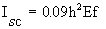 (Equation 9.5)
where h is the height in meters, E is the
E-field magnitude in kilovolts per meter, f is the frequency
in kilohertz, and is in milliamperes.
Deno (1977) measured the short-circuit current and the
distribution of current at 60 Hz in a metallized mannequin
consisting of insulated material covered with copper foil.
Breaks in the copper foil were used to measure current
distribution. By measuring short-circuit currents near
powerful VLF-MF transmitting stations, Guy and Chou (1982)
showed that the determination of currents at 60 Hz is
applicable to the VLF-MF band.
Gandhi and Chatterjee (1982) used a Norton's equivalent
circuit to represent the body and from it calculated the
total current in the human body to be
 (Equation 9.6)
where  is leakage resistance of the body to
ground, and
is leakage resistance of the body to
ground, and  and
and  are equivalent body resistance and
capacitance respectively. Combining Equations 9.6 and 9.4
gives the current in a person exposed to an electric field,
E.
are equivalent body resistance and
capacitance respectively. Combining Equations 9.6 and 9.4
gives the current in a person exposed to an electric field,
E.
Figure 9.1.
Relationship between effective area and
short-circuit current () for exposed human figure (Guy
and Chou, 1982).
9.1.2. Measurement of Body Potential and
Dimensions
In baboons the equipotential planes occur perpendicular
to the long axis of the body when the incident E-field
is parallel to the long axis (Frazier et al. , 1978; Bridges
and Frazier, 1979), so the potential distribution inside the
body can be predicted from the surface potential. While
applying a harmless low-level VLF current through volunteers'
bodies, Guy and Chou (1982) measured the surface potential
distribution. They measured the circumference and maximum
dimensions of the subject's body and limbs as a function of
position every 5 cm from the feet to the head, and then
assumed an elliptical cross section to determine the cross-sectional area. The
sum of the volumes of those elliptical cylinders was compared
to the body volume to check the accuracy of the measurements.
The body volume was calculated from body weight by assuming a
specific gravity of 1.06.
9.1.3. Calculation of Body Resistance and SAR
From the information obtained in the body potential
measurements described above, Guy and Chou (1982) calculated
the electrical conductivity and the resistance per unit
length for various regions of the body. The resistance
between two equipotential planes perpendicular to the axis of
the body or body member is given by
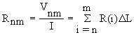 (Equation 9.7)
where  is the measured potential difference,
I is the applied current,
is the measured potential difference,
I is the applied current,  is the incremental distance, and
R(i) is the resistance per unit length of the length. The
conductivity of a particular region of the body is related to
R(i) by
is the incremental distance, and
R(i) is the resistance per unit length of the length. The
conductivity of a particular region of the body is related to
R(i) by
 (Equation 9.8)
where A(i) is the cross-sectional area of the
ith section. Combining Equations 9.8 and 9.7 and solving for
 gives
gives
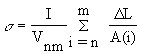 (Equation 9.9)
where is the effective conductivity in the
region between the equipotential planes where Vnm is
measured. Once a has been determined, the potential
distribution [V(k)], the current density [J(i)], and the
local SAR [SAR(i)] may be obtained for any known current
distribution [I(i)] from the following equations:
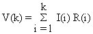 (Equation 9.10)
J(i)=I(i)/A(i) (Equaiton 9.11)
(Equation 9.10)
J(i)=I(i)/A(i) (Equaiton 9.11)
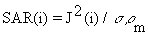 (Equation 9.12)
where  is the density of the tissue (usually
assumed to be equal to unity). Regional and whole-body power
absorption can be found from
is the density of the tissue (usually
assumed to be equal to unity). Regional and whole-body power
absorption can be found from
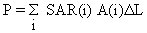 (Equation 9.13)
9.2. CALCULATED AND MEASURED DATA
Figures 9.2-9.4 show Guy and Chou's (1982) plots of
Deno's measured distributions of surface currents on
copper-foil-covered mannequins. In the data shown in Figures
9.2 and 9.3, Deno had not measured the current distribution
in the arm but reported it as 14% of the short-circuit
current. Guy and Chou assumed a cosine distribution for their
plots. In Figure 9.2, the maximum current occurs at the feet,
with a value given by Equation 9.5. From Figure 9.3, the
maximum current for a man exposed in free space is given
by
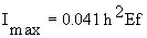 (Equation 9.14)
(same units as Equation 9.5), and from Figure
9.4, with feet insulated but a hand grounded, by
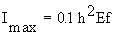 (Equation 9.15)
Figure 9.2.
Relative surface-current distribution in
grounded man exposed to VLF-MF fields [after Deno, 1977 (Guy
and Chou, 1982)].
Figure 9.3.
Relative surface-current distribution in man
exposed in free space to VLF-MF electric fields [after Deno,
1977 (Guy and Chou, 1982)].
Figure 9.4.
Relative surface-current distribution in man
exposed to VLF-MF electric fields with feet insulated and
hand grounded [after Deno, 1977 (Guy and Chou, 1982)].
Tables 9.1 and 9.2 summarize, respectively, the effects
of currents on humans and some values specified in safety
standards. Table 9.3 gives currents in various parts of the
body, based on 60-Hz work by Kaune (1980). Table 9.4 gives
short-circuit currents for various objects exposed to VLF-MF
fields, based on 60-Hz work. Tables 9.5-9.7 show data
measured in VLF-MF fields. The plot of these data in Figure
9.5 compares very well with values calculated from Equation
9.5
Table 9.1.
Summary Of Electric-Current Effects On Humans (Guy and Chou, 1982)
Table 9.2.
Maximum 60-Hz Currents Allowed To Human Body By National Electrical Code (mA) And Equivalent Levels At Other Frequencies (Guy and Chou, 1982)
Table 9.3.
Current And Current Density In Man Exposed To VLF-MF [f(kHz)] 1-kV/m Electric Fields (based on Kaune, 1980)
(Guy and Ghou, 1982)
Table 9.4.
Short-Circuit Currents For Objects Exposed To VLF-MF [f(kHz)] 1-kV/m Electric Fields (Guy and Chou, 1982)
Table 9.5.
Comparison Of Measured And Theoretical
Short-Circuit Body Current For Man Exposed To VLF-MF Electric Fields With Feet Grounded (Guy and Chou, 1982)
Table 9.6.
Measured Body Currents [mA/(kv/m)] To Ground For Subjects Exposed Under Different Conditions To 24.8-kHz VLF Electric Fields [Washington VLF (Guy and Chou, 1982)]
Table 9.7.
Comparison Of Measured And Theoretical
Person-To-VehicleCurrent Resulting From VLF-MF Electric-Field Exposure (Guy and Chou, 1982)
Figure 9.5.
Comparison of theoretical and measured
short-circuit body current of grounded man exposed to VLF-IAF
electric field that is parallel to body axis (Guy and Chou,1982).
Figures 9.6-9.8 show results by Gandhi and Chatterjee
(1982) of human body resistance, threshold perception and
let-go currents and corresponding unperturbed incident
E-fields that would produce these threshold currents for
various conditions. Perception current is defined as the
smallest current at which a person feels a tingling or
pricking sensation due to nerve stimulation. Let-go current
is defined as the maximum current at which a human is still
capable of releasing an energized conductor using muscles
directly stimulated by that current. Tables 9.8-9.10 show
values of threshold perception measured with an experimental
setup like the one illustrated in Figure 9.9. Either a
copper-disk or a brass-rod electrode was used in the
measurements. Table 9.11 gives calculated values of currents
through the wrist and finger for a maximum SAR of 8 W/kg.
Table 9.12 shows the body dimensions calculated by Guy
and Chou for one person. Figures 9.10-9.17 show their
calculated current distributions for the current
distributions of Figures 9.2-9.4. The data in Figures
9.10-9.17 are for exposure of a subject with feet
electrically grounded, in free space, with feet insulated but
hands grounded, and with feet grounded but one hand
contacting a large object such as a vehicle. To calculate
values of current, current density, and potential in a
subject contacting one of the specific objects in Table 9.4,
multiply the values in Figures 9.10-9.17 by the shortcircuit
object currents in Table 9.4. Calculations for objects not
given in Table 9.4 can be made by looking up methods for
calculating the effective surface area, S, in the literature
(for example, Deno, 1977; Transmission-Line Reference Book,
1979) using Equation 9.5 to calculate , and proceeding as
described above.
Figure 9.6.
Average values of the human body resistance,
Rh, (see Equation 9.6) assumed for the range 10 kHz to 20 MHz
(Gandhi and Chatterjee, 1982).
Figure 9.7.
Perception and let-go currents for finger
contact for a 50th percentile human as a function of
frequency assumed for the calculations (Gandhi and
Chatterjee, 1982). [These were obtained as a composite of the
experimental data of Dalziel and Mansfield (1950), Dalziel
and Lee (1969), and Rogers (1981).]
Figure 9.8.
Unperturbed incident E-field
required to create threshold perception and let-go currents in a human for conductive
finger contact with various metallic objects, as a function of frequency (Gandhi and
Chatterjee, 1982)
Table 9.8.
Threshold Currents For Perception When In Contact With The Copper-Plate Electrode And Threshold Incident Electric Fields For Perception When In
Contact With Various Metal Objects (Gandhi et al., 1984)
Table 9.9.
Statistical Analysis Of Measured Data On
Threshold Currents For Perception With Subjects Barefoot And With The Wristband (Gandhi et al., 1984)
Table 9.10.
Threshold Currents For Perception When In Grasping Contact With The Brass-Rod Electrode And Threshold External Electric Fields For Perception When In Contact With A Compact Car (Cg = 800 pF) (Gandhi et al., 1984)
Figure 9.9.
Experimental arrangement for measuring
threshold currents for perception and let-go (Gandhi and Chatterjee,
1982).
Table 9.11.
Currents Through The Wrist And Finger For Maximum SAR = 8 W/kg. (Cross-sectional areas are for nonbony regions of respective parts of the body.) (Gandhi et al., 1984)
Table 9.12.
Dimensions Of Body Used For VLF-MF Exposure Model (Guy and Chou, 1982)
Figure 9.10.
Calculated current distributions as a function of a position in man exposed to 1-kV/m VLF-MF
fields with feet grounded (Guy and Chou, 1982)
Figure 9.11.
Calculated current density flowing through one arm. The exposure is the same as that of Figure 9.10 (Guy and Chou, 1982).
Figure 9.12.
Calculated current distribution as a function of position in
man exposed to 1-kv/m VLF-MF fields in free space (Guy and Chou, 1982).
Figure 9.13.
Calculated current density flowing through one arm. The exposure condition is the same as
for Figure 9.12 (Guy and Chou, 1982).
Figure 9.14.
Calculated current distribution as a function of position in
man exposed to 1-kv/m VLF-MF fields with feet insulated but hands grounded (Guy and Chou, 1982).
Figure 9.15.
Calculated current density flowing through one arm. The exposure condition is the same as
for Figure 9.14 (Guy and Chou, 1982).
Figure 9.16.
Calculated current distribution as a function of position in man with hand contacting a large object and with feet grounded. A 1-mA current is assumed to floating throughb the arm, thorax, and legs of the subject to the ground, F=60 Hz (Guy and Chou, 1982).
Figure 9.17.
Calculated current density flowing through one arm. The exposure condition is the same as for Figure 9.16 (Guy and Chou, 1982).
Table 9.13 gives regional and average SARs for various
exposure conditions. Figure 9.18 shows measured values of the
imaginary component of the permittivity (Tables 9.14 and
9.15; see Section 3.2.6 for the relationships of
permittivity, conductivity, and loss factor) along with
values of the real and imaginary components given in the
first edition of this handbook. Figures 9.19 and 9.20 show
average SARs of Table 9.13 compared with theoretical values.
Further power absorption calculations are given in Table
9.16.
Figure 9.21 shows the maximum electric-field strength
below levels of 1000 V/m that would violate any of the
following conditions:
- The maximum current through any body member contacting
ground or an object should not exceed levels equivalent to
those allowed by the National Electric Safety Code in the
frequency range where shock hazards may occur.
- Total possible current entering the body should not
exceed 200 mA, for prevention of RF burns.
- The 0.4-W/kg average and 8-W/kg maximum SAR
recommended by the ANSI C95.1-1982 Standard shall not be
exceeded.
According to the calculated data of Guy and Chou (1982),
none of the conditions would be violated for exposure of
persons isolated in free space at E-field strengths of 1 kV/m
or below. Other conditions are shown in Figure 9.21.
Table 9.13.
Distribution Of Power Absorption (Watts)In Man Exposed To VLF-MF Fields: 1-kV/m Exposure, E-Field
Parallel Long Axis, 1-mACurrent Assumed For Contact With Object (Guy and Chou, 1982)
Figure 9.18.
Real part,  ', and imaginary part,",
of the dielectric constant for high-water-content tissue. The
dashed line is measured values (Guy and Chou, 1982) The
other lines are values given in the first edition of this
handbook
', and imaginary part,",
of the dielectric constant for high-water-content tissue. The
dashed line is measured values (Guy and Chou, 1982) The
other lines are values given in the first edition of this
handbook
Table 9.14.
Average Apparent Conductivity Of Man Based On Whole-Body In Vivo Measurements(S/m) (Guy and Chou, 1982)
Table 9.15.
Average Apparent Loss Factor Of Man Based On Whole-Body In Vivo Measurements (Guy and Chou, 1982)
Figure 9.19.
Comparison of calculated average SAR
(obtained from VLF analysis) with average SAR (reported in
the first edition of this handbook) of average absorbed power
in an ellipsoidal model of an average man (Guy and Chou,
1982).
Figure 9.20.
Comparison of theoretical and experimentally
measured whole-body average SAR for realistic man models
exposed at various frequencies. The experimental curve is
measured results in scaled human-shaped models at simulated
VLF frequencies (Guy and Chou, 1982).
Table 9.16.
Distribution Of Power Absorption (Watts) In Man, With Feet Grounded, Exposed To 1-kV/m VLF-MF Fields While In Contact With Vehicle (Guy and Chou, 1982)
Figure 9.21.
Required restrictions of VLF-MF
electric-field strength to prevent biological hazards related to shock, RF
burns, and SAR exceeding ANSI C95.1 criteria (Guy and Chou,
1982).

Go to Chapter 10.
Return to Table of Contents.
Last modified: June 14, 1997
© October 1986, USAF School of Aerospace Medicine,
Aerospace Medical Division (AFSC), Brooks Air Force Base,
TX 78235-5301