 |
Radiofrequency Radiation
|
|
Radiofrequency Radiation
|
Experimental data from the literature on the average SAR, SAR distributions, and the temperature-rise distributions on some test animals, human subjects, and phantom models, along with some calculated data, are shown in Figures 8.1-8.47 and Tables 8.1-8.4. References are given in the figure captions and table headings.
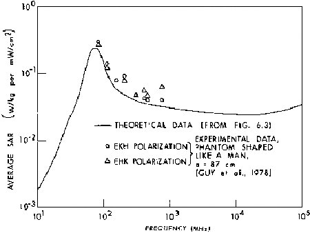
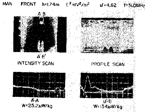
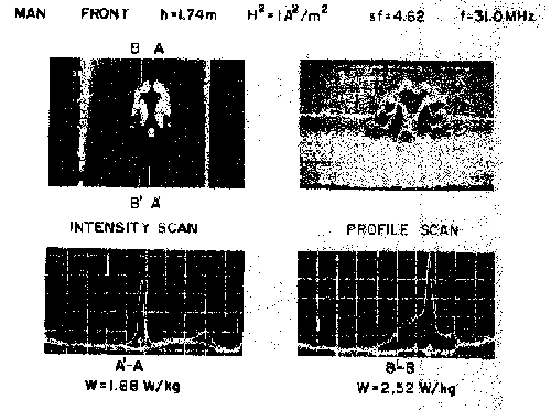
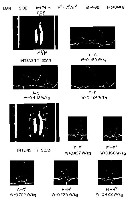
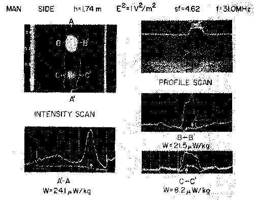
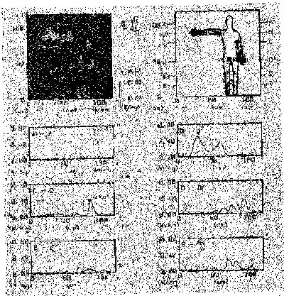
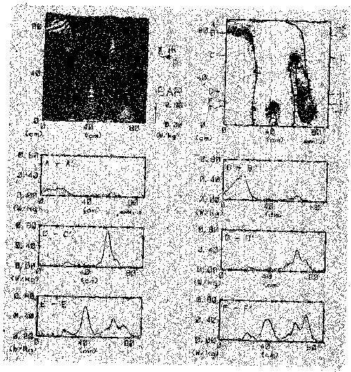
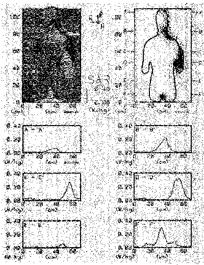
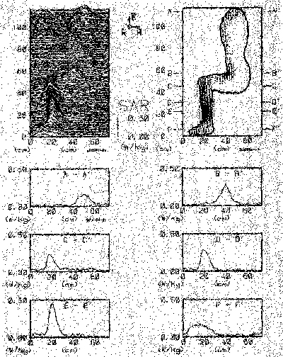
A possible explanation of the higher values lies in the very nonuniform distribution of SAR within the body, as explored extensively with thermographic techniques by Guy et al. (1976b, 1984) and illustrated by Figures 8.32 to 8.46. Measured local SAR values are as much as 13 times greater than average SAR values at 450 MHz. In particular the legs, which are relatively thinner and longer than the main trunk of the body, absorb significantly more than the average (see Figures 8.36, 8.46); the reason is explained qualitatively in Section 5.1.5. Since using pulse functions with the moment method to calculate local SAR in block models has been unsatisfactory (Massoudi et al., 1984), average-SAR calculation by the same method may not adequately include the higher local absorption in the legs, thus resulting in lower values of average SAR. Calculated average SARs in prolate spheroidal models, which are very close to those calculated in the block model, also would not account for higher absorption in the legs. Thus the calculated average SARs in both block and spheroidal models might be low because the calculations do not adequately include locally high SAR values. More calculated and measured values are needed to clarify the results.
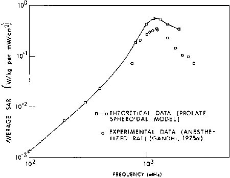
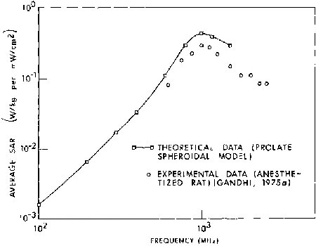
Figure 8.3.
Calculated and measured values of the average
SAR for prolate spheroidal phantom of a sitting rhesus monkey; a
= 0.2 m, b = 6.46 cm, V = 3.5 x 10 -3m3 (Allen et al.,
1975).
Figure 8.4.
Measured values of the average SAR for a
live, sitting rhesus monkey, for six standard polarizations
(Allen et al., 1976).
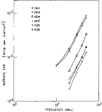
Figure 8.5.
Measured values of the average SAR for saline-filled ellipsoidal phantoms, for six standard
polarizations; a = 20 cm, b = 7.92 cm, c = 5.28 cm,  = 0.64 S/m (Allen et al., 1976).
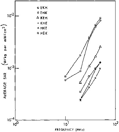
Figure 8.6.
Measured values of the average SAR for
saline-filled ellipsoidal phantoms, for six standard
polarizations; a = 20 cm, b = 7.92 cm, c = 5.28 cm, = 0.54
S/m (Allen et al., 1976).
Figure 8.7.
Measured values of the average SAR for
saline-filled ellipsoidal phantoms, for six standard
polarizations; a = 20 cm, b = 7.92 cm, c = 5.28 cm, = 0.36
S/m (Allen et al., 1976).
Figure 8.8.
Calculated and measured values of the average
SAR for models of an average man, E polarization.
Figure 8.9.
Calculated and measured values of the
average SAR for a 96-g rat, K polarization.
Figure 8.10.
Calculated and measured values of
the average SAR for a 158-g rat, K polarization.
Figure 8.11.
Calculated and measured values of
the average SAR for a 261-g rat, K polarization.
Figure 8.12.
Calculated and measured values of
the average SAR for a 390-g rat, K polarization.
Figure 8.13.
Calculated and measured values of the
average SAR for models of a rat, H polarization.
Figure 8.14.
Calculated and measured values of the
average SAR for models of a rat, K polarization.
Figure 8.15.
Calculated and measured values of the
average SAR for models of a rat, E polarization.
Figure 8.16.
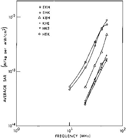
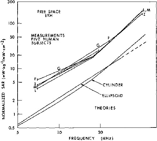
Comparison of free-space absorption rates of
five human subjects with each other and with two standard
theories (Hill, 1984).
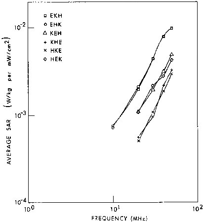
Figure 8.17.
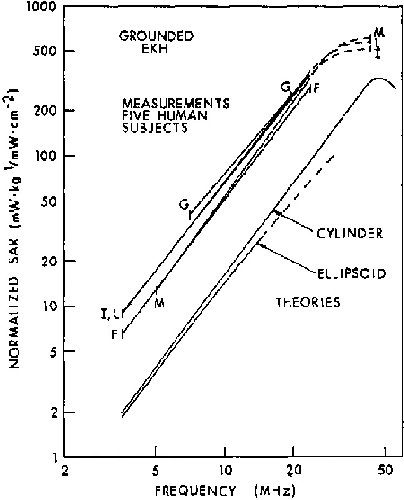
Comparison of the grounded absorption rates
of five human subjects with each other and with two standard
theories (Hill, 1984).
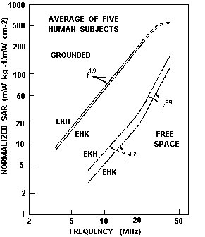
Figure 8.18.
The frequency dependence of the average
absorption rates for five human subjects in the EKH and EHK
orientations under both free-space and grounded conditions
(Hill, 1984).
Figure 8.19.
Measured relative SARs in scaled saline
spheroidal models of man. To emphasize the differences in the
absorption characteristics, the values are normalized with
respect to their far-field value at d/![]() = 0.5.
= 0.5. ![]() T is the
temperature rise in the saline solution after exposure for
time t (Iskander et al., 1981).
T is the
temperature rise in the saline solution after exposure for
time t (Iskander et al., 1981).
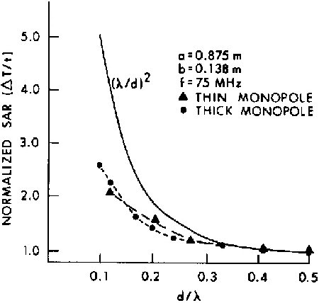
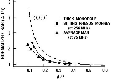
Figure 8.20
Measured relative SARs in scaled saline spheroidal models versus distance. SAR values for the
different models are normalized with respect to their
planewave value. ![]() T is the temperature rise in the saline
solution after exposure for time t (Iskander et al.,
1981).
T is the temperature rise in the saline
solution after exposure for time t (Iskander et al.,
1981).
Figure 8.21. 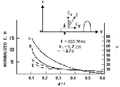
Measured relative fields versus distance for
the thick monopole on a ground plane. The values of E and H
are normalized with respect to their values at d/![]() = 0.6
(Iskander et al., 1981).
= 0.6
(Iskander et al., 1981).
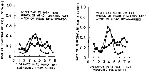
Figures 8.25 and 8.26.
Rate of temperature rise from RFR exposure
in the face of detached M. mulatta head; 1.2 GHz, CW, 70
mW/cm² far field Burr and Krupp, 1980).
Figure 8.26.
Rate of temperature rise from RFR exposure
at the right side of a detached M. mulatta head; 1.2 GHz, 70
mW/cm² CW, far field (Burr and Krupp, 1980).
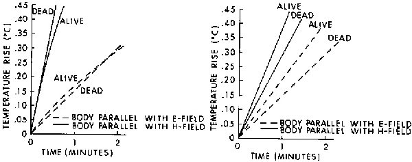
Figures 8.27 and 8.28.
Rate of temperature rise from RFR exposure
at the back of detached M. mulatta head; 1.2 GHz, CW, 70
mW/cm² , far field (Burr and Krupp, 1980).
Figure 8.28.
Rate of temperature rise from RFR exposure
to the back of an M. mulatta cadaver head (with body
attached); 1.2 GHz, CW, 70 mW/cm², far field.Temperature
rise shown for animal's body oriented parallel with the E-
and H-fields (Burr and Krupp, 1980).
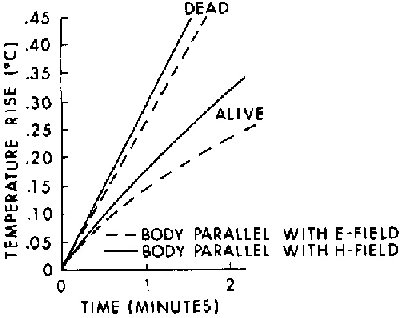
Figures 8.29 and 8.30.
Temperature rise (at 2.0 cm into the top of
the head) of an M. mulatta exposed to 70 mW/cm², 1.2
GHz, CW, RFR, in the far field (Burr and Krupp, 1980).
Figure 8.30.
Temperature rise (at 3.5 cm into the top of
the head) of an M. mulatta exposed to 70 mW/cm², 1.2
GHz, CW, RFR in the far field (Burr and Krupp, 1980).
Figure 8.31.
Temperature rise (at 3.5 cin into the back of
the head) of an M. mulatta exposed to 70 mW/cm², 1.2 GHz,
CW, RFR, in the far field (Burr and Krupp, 1980).
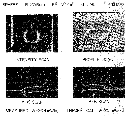
Figure 8.32.
Thermographic results of exposing a
4.3-cm-radius sphere to 144-MHz TM110 electric field in a
rectangular resonant cavity simulating a 25.6-cm-radius
sphere exposed to 24.1 MHz: vertical divergence = 2°C,
horizontal divergence = 2 cm (Guy et al., 1976b) ( ©
1976 IEEE)
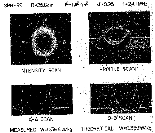
Figure 8.33.
Thermographic results of exposing a
4.3-cm-radius sphere to 144-MHz TE102 magnetic field in a
rectangular resonant cavity simulating a 25.6-cm-radius
sphere exposed to 24.1 MHz: vertical divergence = 2°C,
horizontal divergence = 2 cm (Guy et al., 1976b) ( ©
1976 IEEE)
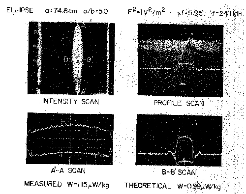
Figure 8.34.
Scale-model thermograms and calculated peak
SAR for 70-kg, 5/1 prolate spheroid (a = 74.8 cm) exposed to
24.1-MHz electric field parallel to major axis: vertical
divergence 2ºC, horizontal divergence = 2.65 cm (Guy et
al., 1976b) ( © 1976 IEEE).
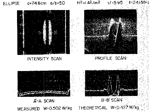
Figure 8.35.
Scale-model thermograms and calculated peak SAR for 70-kg, 5/1 prolate spheroid (a = 74.8 cm) exposed to
24.1-MHz magnetic field parallel to major axis: vertical
divergence 2ºC, horizontal divergence = 2.65 cm (Guy et
al., 1976b) ( © 1976 IEEE)
Figure 8.36.
Scale-model thermograms and measured peak SAR for 70-kg, 1.74-m-height frontal-plane man model exposed to
31.0-MHz electric field parallel to the long axis: vertical
divergence = 2ºC, horizontal divergence = 4 cm (Guy et
al., 1976b) ( © 1976 IEEE).
Figure 8.37.
Scale-model thermograms and measured peak SAR for 70-kg, 1.74-m-height frontal-plane man model exposed to
31.0-MHz magnetic field perpendicular to the major axis:
vertical divergence = 2ºC, horizontal divergence = 4 cm
(Guy et al., 1976b) (© 1976 IEEE).
Figure 8.38.
Scale-model thermograms and measured peak SAR for 70-kg, 1.74-m-height medial-plane man model exposed to 31.0-MHz magnetic field perpendicular to the median plane: vertical divergence = 2ºC, horizontal divergence = 2.65 cm
(Guy et al., 1976b) ( © 1976 IEEE)
Figure 8.39.
Scale-model thermograms and measured peak SAR for 70-kg, 1.74-m-height medial-plane man model exposed to 31.0-MHz electric field parallel to the major axis: vertical divergence = 2º C, horizontal divergence = 2.65 cm (Guy
et al., 1976b) (© 1976 IEEE).
Figure 8.40.
Computer-processed whole-body thermograms expressing SAR patterns for man with arms up, exposed to 1-mW/cm² 450 MHz radiation with EHK polarization (Guy et al., 1984) (© 1984 IEEE).
Figure 8.41.
Computer-processed whole-body thermograms
expressing SAR patterns for man with one arm extended,
exposed to 1-mW/cm² 450 MHz radiation with KEH
polarization (Guy et al., 1984) (© 1984 IEEE).
Figure 8.42.
Computer-processed upper-body thermograms
expressing SAR patterns for man with one arm extended,
exposed to 1-mW/cm² 450 MHz radiation with KEH
polarization (Guy et al., 1984) (© 1984 IEEE).
Figure 8.43.
Computer-processed midbody thermograms
expressing SAR patterns for man with one arm extended,
exposed to 1-mW/cm² 450 MHz radiation with KEH
polarization (Guy et al., 1984) (© 1984 IEEE).
Figure 8.44.
Computer-processed lower-body thermograms
expressing SAR patterns for man with one arm extended,
exposed to 1-mW/cm² 450 MHz radiation with KEH
polarization (Guy et al., 1984) (© 1984 IEEE).
Figure 8.45.
Computer-processed whole-body thermograms
expressing SAR patterns for man sitting (frontal plane),
exposed to 1-mW/cm² 450 MHz radiation with EKH
polarization (Guy et al., 1984) (© 1984 IEEE).
Figure 8.46.
Computer-processed whole-body thermograms
expressing SAR patterns for man sitting (sagittal plane
through leg), exposed to 1-mW/cm² 450 MHz radiation with
EHK polarization (Guy et al., 1984) (© 1984 IEEE).
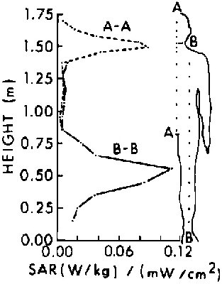
Figure 8.47.
SAR distribution along an average man-model
height for two cross sections; 1-mW/cm² incident-power
density on the surface of the model, frequency 350 MHz E||L,
K back to front (Krazewski et al., 1984) (© 1984
IEEE).
Go to Chapter 9.
Return to Table of Contents.
Last modified: June 14, 1997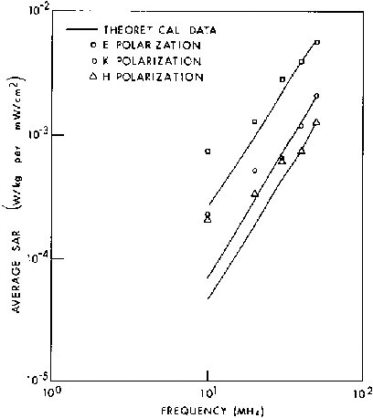