 |
Radiofrequency Radiation
|
|
Radiofrequency Radiation
|
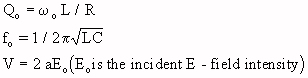
Figure 5.1.
Illustration of different techniques, with their frequency limits, used for calculating SAR data for
models of an average man.
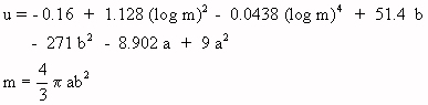
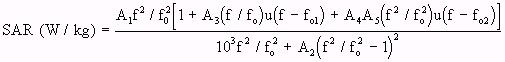 (Equation 5.1)
where (as given by Equations 5.5 - 5.9) A1, A2, A3, and A4
are functions of a and b, and A5 is a function of ![]() . Unit
step function u (f - f ol ) is defined by
. Unit
step function u (f - f ol ) is defined by
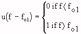
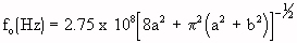
and u (f - f o2 ) is similarly defined. Also, fo < fol < fo2. The resonant frequency, fo , is given by the following empirical relation:
 (Equation 5.2)
![]() (Equation 5.3)
(Equation 5.3)
![]() (Equation 5.4)
(Equation 5.4)
A1 = -0.994 - 10.690 a + 0.172 a/b + 0.739 a-1 + 5.660 a/b2 (Equation 5.5)
A2 = -0.914 + 41.400 a + 399.170 a/b - 1.190 a-1 -2.141 a/b2 ((Equation 5.6)
A3 = 4.822 a - 0.084 a/b - 8.733 a2 + 0.0016 (a/b)2 + 5.369 a3 (Equation 5.7)
A4 = 0.335 a + 0.075 a/b - 0.804 a2 - 0.0075 (a/b)2 + 0.640 a3 (Equation 5.8)
A5 = |  / 20 | -1/4 (Equation 5.9)
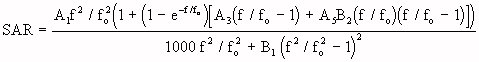
 (Equation 5.10)
where
| (Equation 5.11) | ||
 |
(Equation 5.12) |
and a, b, A1, A2, A4, A5, and fo are as defined previously.
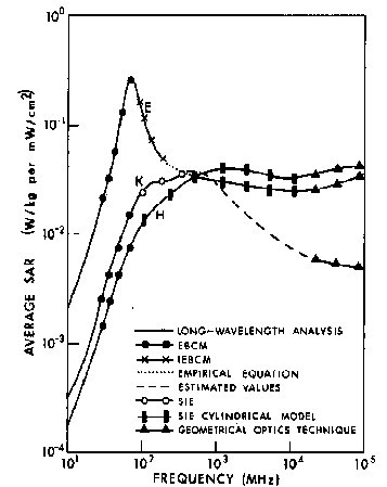
Figure 5.2.
Average SAR calculated by the empirical
formula compared with the curve obtained by other
calculations for a 70-kg man in E polarization. For the
prolate spheroidal model, a = 0.875 m and b = 0.138 m; for
the cylindrical model, the radius of the cylinder is 0.1128 m
and the length is 1.75 m.
Figure 5.2 (continued).
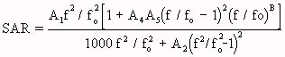
 (Equation 5.13)
where Al, A 3 and A5 are defined in Equations 5.5, 5.7, and 5.9, and
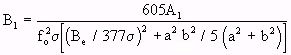 |
(Equation 5.14) |
| (Equation 5.15) | |
| (Equation 5.16) | |
| (Equation 5.17) | |
| (Equation 5.18) |
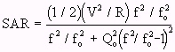 (Equation 5.19)
where
Comparing Equations 5.1 (up to resonance) and 5.19--and keeping in mind that input voltage aEo is applied across the input impedance and the radiation impedance of a monopole rather than a dipole antenna--the parameters R, L, and C of Equation 5.19 can be expressed in terms of Al, A2 and f o. Therefore, we first compute the parameters Al, A2, and fo so that the power calculated from Equation 5.1 will fit (with least-squares error) the numerical results of the SAR in a man model on a ground plane (Hagmann and Gandhi, 1979). The corresponding R, L, and C parameters will hence be valid for a half-spheroid in direct contact with a perfectly conducting ground plane. Introducing a small separation distance between the half-spheroid and the ground plane, in the form of an air gap or a resistive gap representing shoes, will correspond to adding the following Rg and Xg parameters in series with the previously derived resonance circuit:
![]() (Equation 5.20)
(Equation 5.20)
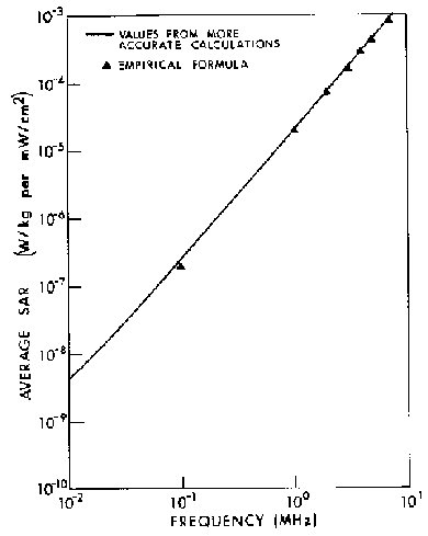
Figure 5.3.
Calculated effect of a capacitive gap, between man model and ground plane, on average SAR.
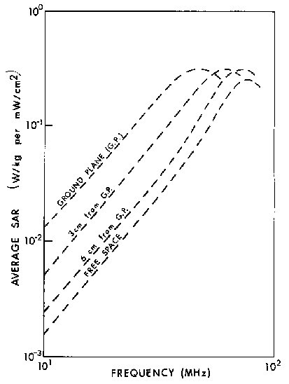
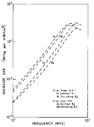
Figure 5.4.
Calculated effect of grounding resistance on
SAR of man model placed at a distance from ground plane.
 (Equation 5.21)
The number N is selected so that
![]() (Equation 5.22)
(Equation 5.22)
where PM is the total power absorbed in the object, given by
 (Equation 5.23)
Then the volume fraction VF is defined as that fraction of the volume in which 90% of the power is absorbed:
![]() (Equation 5.24)
(Equation 5.24)
Go to Chapter 5.1.2
Return to Table of Contents.
Last modified: June 14, 1997
© October 1986, USAF School of Aerospace Medicine, Aerospace Medical Division (AFSC), Brooks Air Force Base, TX 78235-5301