5.1.3. Sensitivity of SAR Calculations to Permittivity Changes
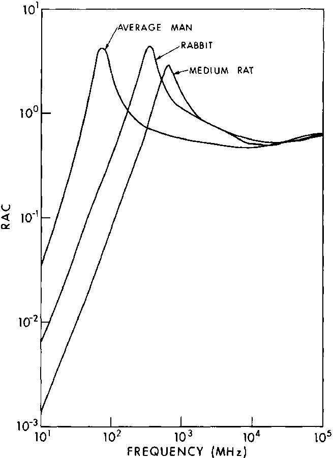
5.1.4. Relative Absorption Cross Section
 (Equation 5.25)
where Pin is the incident power density and M is the mass of the object exposed to EM fields.
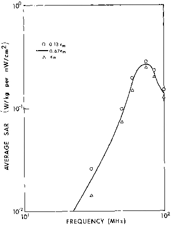
Figure 5.7.
Calculated average SAR in a prolate
spheroidal model of an average man, as a function of
frequency for several values of permittivity. ![]() m is the
permittivity of muscle tissue.
m is the
permittivity of muscle tissue.
 (Equation 5.26)
 (Equation 5.27)
Figure 5.8.
Relative absorption cross section in prolate
spheroidal models of an average man, a rabbit, and a
medium-sized rat--as a function of frequency for E
polarization.
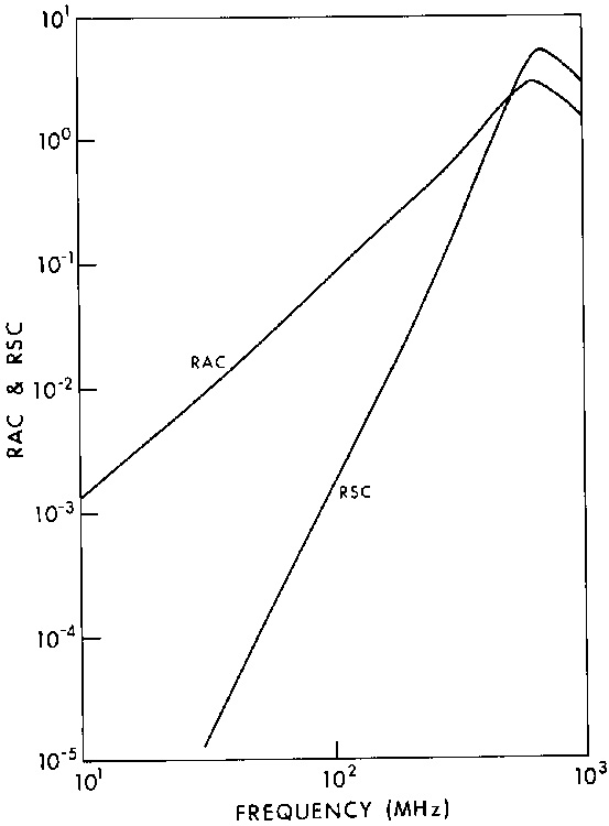
Figure 5.9.
Comparison of relative scattering cross
section (RSC) and relative absorption cross section (RAC) in
a prolate spheroidal model of a medium rat--for planewave
irradiation, E polarization.
5.1.5. Qualitative Dosimetry
E1p = E2p (Equation 5.28)
 1E1n = 2E2n (Equation 5.29)
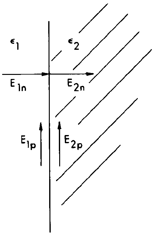
where Elp and E2p are components parallel to the
boundary, and Eln and E2n are component, perpendicular to the
boundary, as shown in Figure 5.10. It is important to
remember that Equations 5.28 and 5.29 are valid only at a
point on the boundary. From Equation 5.29, we can see that
E2n = 1 Eln /2; and if 2 >> 1, then E2n << E1n. Thus if Eln is the field in free space and E2n is the field in an absorber, the internal field at the boundary will be much weaker than the external field at the boundary when 2 > > 1 and the fields are normal to the boundary. Also, from Equation 5.28, we see that the external field and the internal field at the boundary are equal when the fields are parallel to the boundary. These two results will be used extensively in explaining relative energy absorption.
Figure 5.10.
Field components at a boundary between two media having different complex permittivities, 1 and 2.
![]() (Equation 5.30)
(Equation 5.30)
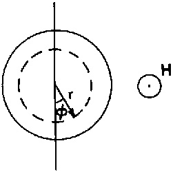
For the very special case of a lossy dielectric cylinder
in a uniform H-field Equation 5.30 can be solved by deducing
from the symmetry of the cylinder and fields that E will have
only a ![]() component that will be constant around a circular
path, such as the one shown dotted in Figure 5.11. For E
constant along the circular path, and H uniform, Equation
5.30 reduces to
component that will be constant around a circular
path, such as the one shown dotted in Figure 5.11. For E
constant along the circular path, and H uniform, Equation
5.30 reduces to
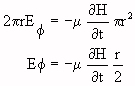 (Equation 5.31)
Thus, Equation 5.30 shows that E is related to the rate of change of the magnetic flux intercepted by the object; and Equation 5.31 shows that for the very special case of Figure 5.11, the E-field circulates around the H-field and is directly proportional to the radius. For this example the circulating E-field (which produces a circulating current) would be larger for a larger cross section intercepted by the H-field. The generalized qualitative relation that follows from Equation 5.30 is that the circulating field is in some sense proportional to the cross-sectional area that intercepts the H-field. This result is very useful in qualitative explanations of relative energy absorption characteristics; however, this qualitative explanation cannot be used indiscriminantly.
Figure 5.11.
A lossy dielectric cylinder in a uniform magnetic field.
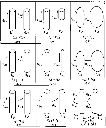
Ein = E e+ Eh (Equation 5.32)
where
QP1.
Ee is stronger when Einc is mostly parallel to the boundary of the object and weaker when Einc is mostly perpendicular to the boundary of the object.
QP2.
Eh is stronger when Hinc intercepts a larger cross section of the object and weaker when Hinc intercepts a smaller cross section of the object.
Figure 5.12.
Qualitative evaluation of the internal
fields based on qualitative principles QPl and QP2. Ee
is the internal E-field generated by Einc, the
incident E-field, and Eh is the internal
E-field generated by Hinc,the incident
H-field.
Table 5.1
Application of QP1 and QP2 To Planewave SARS
 /d)2 , since the magnitude of the E- and H-fields is expected to
increase more rapidly than /d in the near-field region.
However, the reasons for the shape of the SAR curve may be
found from Figure 8.21, which shows the behavior of the
measured fields of the antenna (designated Einc and
Hinc with respect to an absorber). The direction of
the Hinc does not change with d, but the magnitude of
Hinc increases faster than /d for d/ < 0.3. The
direction of Einc however, changes significantly with
d. In the far field, the angle = 0.1, it is
about 70º. According to QP1, this change in angle has a
significant effect on Ee Thus the change in SAR with
d/ results from three factors:
/d)2 , since the magnitude of the E- and H-fields is expected to
increase more rapidly than /d in the near-field region.
However, the reasons for the shape of the SAR curve may be
found from Figure 8.21, which shows the behavior of the
measured fields of the antenna (designated Einc and
Hinc with respect to an absorber). The direction of
the Hinc does not change with d, but the magnitude of
Hinc increases faster than /d for d/ < 0.3. The
direction of Einc however, changes significantly with
d. In the far field, the angle = 0.1, it is
about 70º. According to QP1, this change in angle has a
significant effect on Ee Thus the change in SAR with
d/ results from three factors:
- Ee increases as the magnitude of Einc increases.
- Ee decreases as
 increases.
- Eh increases as the magnitude of Hinc increases.
/d, Ee increases much more slowly than /d because of the
combination of factors 1 and 2. The average SAR, which is
proportional to E2in does not increase as fast as (/d)2
because Ee affects Ein more than Eh
does. On the other hand, since the monkey-size spheroid is
relatively shorter and fatter than the man-size spheroid,
Eh has a stronger effect on Ein for the monkey
than for the man. Consequently, the SAR for the monkey
increases more rapidly as d decreases than does the SAR for
the man.
. The reasons for this
can be seen from Figures 6.37 - 6.39:
- Einc is slightly lower at 200 MHz and significantly lower at 300 MHz than at the other frequencies.
- Hinc is lower at 200 and 300 MHz than at the other frequencies.
- The angle of Einc with the z axis is
significantly higher at 200 and 300 MHz than at the other
frequencies.
. According to QP1, as increases, the SAR
decreases. The effect of can be seen from the 300-MHz
curve which begins to rise rapidly at y/ = 0.3, where
decreases steeply. A surprising aspect of the correspondence
between incident-field characteristics and the relative SAR
characteristics is that the correlation was based on the
values of the incident fields at only one point in space.
/y (as shown in Figure 6.37) for
0.15 < y/ < 0.5 is slower than /y, the relative
SARs for an absorber at distance d from the dipole for both H
and K polarizations vary faster than (/d)2 in this region
(as seen in Figures 6.32 and 6.33). From the nature of the
incident fields (as shown in Figures 6.37-6.39), Eh
appears to dominate for K and H polarizations, while
Ee dominates for E polarization. The same behavior is
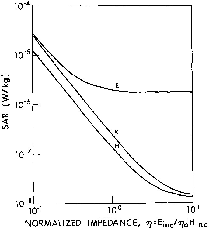
shown in a different way in Figure 5.13, where the calculated
average SAR for a prolate spheroidal model of an average man
is shown as a function of /d)2
variation, as shown in Figures 6.32 and 6.33.
Figure 5.13.
Average SAR in a prolate spheroidal model of
an average man as a function of normalized impedance for each
of the three polarizations. (a = 0.875 m, b = 0.138 m, f =
27.12 MHz,  = 0.4 S/m, incident E-field is 1
V/m.)
= 0.4 S/m, incident E-field is 1
V/m.)
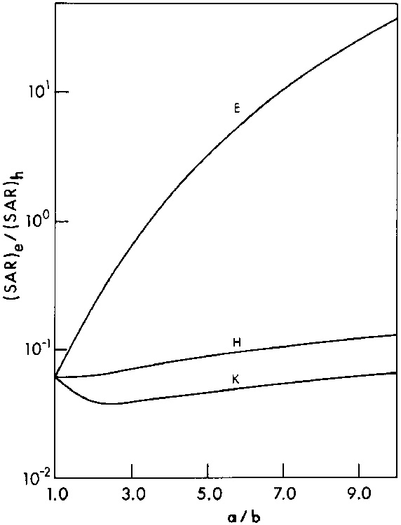
Figure 5.14.
Ratio of (SAR)e, to (SAR)h of a 0.07-m3
prolate spheroid for each polarization as a function of the
ratio of the major axis to the minor axis of the spheroid at
27.12 MHz, = 0.4 S/m.
Go to Chapter 5.2
Return to Table of Contents.
Last modified: June 14, 1997
© October 1986, USAF School of Aerospace Medicine, Aerospace Medical Division (AFSC), Brooks Air Force Base, TX 78235-5301