3.2.8. Wave Solutions to Maxwell's Equations


One class of solutions to Maxwell's equations results in wave descriptions of the electric and magnetic fields. When the frequency of the source charges or currents is high enough, the E- and B-fields produced by these sources will radiate out from them. A convenient and commonly used description of this radiation is wave propagation. Although a wave description of electromagnetic fields is not necessary, it has many advantages. The basic ideas of wave propagation are illustrated in Figures 3.16 and 3.17. Electromagnetic wave propagation is analogous to water waves rolling in on a beach. As shown in Figure 3.16, the distance from one crest to the next (in meters or some other appropriate unit of length) is defined as the wavelength, which is usually designated as . The velocity of propagation is the velocity at which the wave is traveling and (from Figure 3.16) is equal to the distance traveled divided by the time it took to travel:

(Equation 3.25 )

Figure 3.16 and Figure 3.17
Figure 3.16. Snapshots of a traveling wave at two instants of time, t1 and t2.
Figure 3.17. The variation of E at one point in space as a function of time.

A detector at one point in space would observe a function that oscillated with time as the wave passed by. This is like someone standing on the beach and watching the wave go by. The height of the water above some reference plane would change with time, as in Figure 3.17. The peak value of the crest is called the wave's amplitude; in Figure 3.17, the peak value (amplitude) is 10 V/m.
Another important value is that of the period, T, of the oscillation, which is defined as the time between corresponding points on the function (see Figure 3.17). The frequency, f, is defined as

f = 1/T (Equation 3.26 )

The units of T are seconds; those of f are hertz (equivalent to cycles per second). The frequency of a water wave could be obtained by standing in one place and counting the number of crests (or troughs) that passed by in 1 s.
For convenience in power relationships (as explained in Section 3.2.6), the rms value of a function is defined. For a given periodic function, f(t), the rms value, F, is

(Equation 3.27 )

where T is the period of the function and to is any value of t. Equation 3.27 shows that the rms value is obtained by squaring the function, integrating the square of the function over any period, dividing by the period, and taking the square root. Integrating over a period is equivalent to calculating the area between the function, f2, and the t axis. Dividing this area by T is equivalent to calculating the average, or mean, of f2 over one period. For example, the rms value of the f(t) shown in Figure 3.18 is calculated as follows: The area between the f2 (t) curve and the t axis between t o and t o + T is (25 x 30) + (4 x 10) = 790; hence the rms value of f is

Figure 3.18
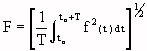
(a) A given periodic function [ f ( t ) ] versus time (t).
(b) The square of the function [ f2 ( t )] versus time.

The rms value of a sinusoid is given by

(Equation 3.28 )

where gp is the peak value of the sinusoid.

The quantities defined above are related by the following equation:

(Equation 3.29 )

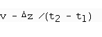
In free space, v is equivalent to the speed of light (c). In a dielectric material the velocity of the wave is slower than that of free space.

Two idealizations of wave propagation are commonly used: spherical waves and planewaves.

Spherical Waves--A spherical wave is a model that represents approximately some electromagnetic waves that occur physically, although no true spherical wave exists. In a spherical wave, wave fronts are spherical surfaces, as illustrated in Figure 3.19. Each crest and each trough is a spherical surface. On every spherical surface, the E- and H-fields have constant values everywhere on the surface. The wave fronts propagate radially outward from the source. (A true spherical wave would have a point source.) E and H are both tangential to the spherical surfaces.

Figure 3.19.
A spherical wave. The wave fronts are spherical surfaces. The wave propagates radially outward in all directions.

Spherical waves have several characteristic properties:
  1. The wave fronts are spheres.
  2. E, B, and the direction of propagation (k) are all mutually perpendicular.
  3. E/H = (called the wave impedance). For free space, E/H = 377 ohms. For the sinusoidal steady-state fields, the wave impedance, , is a complex number that includes losses in the medium in which the wave is traveling.
  4. Both E and H vary as 1/r, where r is the distance from the source.
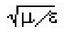
  5. Velocity of propagation is given by v = 1 / .The velocity is less and the wavelength is shorter for a wave propagating in matter than for one propagating in free space. For sinusoidal steady-state fields, the phase velocity is the real part of the complex number 1 / . The imaginary part describes attenuation of the wave caused by losses in the medium.
Planewaves--A planewave is another model that approximately represents some electromagnetic waves, but true planewaves do not exist. Planewaves have characteristics similar to spherical waves:

  1. The wave fronts are planes.
  2. E, H, and the direction of propagation (k) are all mutually perpendicular.
  3. E/H = (called the wave impedance). For free space, E/H = 377 ohms. For the sinusoidal steady-state fields, the wave impedance, , is a complex number that includes losses in the medium in which the wave is traveling.
  4. E and H are constant in any plane perpendicular to k.
  5. Velocity of propagation is given by v = 1/ The velocity is less and the wavelength is shorter for a wave propagating in matter than for one propagating in free space. For sinusoidal steady-state fields, the phase velocity is the real part of the complex number 1/ . The imaginary part describes attenuation of the wave caused by losses in the medium.

Figure 3.20 shows a planewave. E and H could have any directions in the plane as long as they are perpendicular to each other. Far away from its source, a spherical wave can be considered to be approximately a planewave in a limited region of space, because the curvature of the spherical wavefronts is so small that they appear to be almost planar. The source for a true planewave would be a planar source, infinite in extent.

Figure 3.20.
A planewave.

3.2.9. Solutions of Maxwell's Equations Related to Wavelength

Maxwell's equations apply over the entire electromagnetic frequency spectrum. They apply from zero frequency (static fields) through the low frequencies, the RF frequencies, the microwave region of the spectrum, the infrared and visible portions of the spectrum, the ultraviolet frequencies, and even through the x-ray portion of the spectrum. Because they apply over this tremendously wide range of frequencies, Maxwell's equations are powerful but are generally very difficult to solve except for special cases. Consequently, special techniques have been developed for several ranges of the frequency spectrum. The special techniques are each valid in a particular frequency range defined by the relationship between wavelength and the nominal size of the system or objects to which Maxwell's equations are being applied. Let the nominal size of the system (some general approximate measure of the size of the System) be L. For example, if the system included a power transmission line 500 km long, then L would be 500 km; if the system were an electric circuit that would fit on a 1- x 2-m table, then L would be the diagonal of the table, .
Three main special techniques are used for solving Maxwell's equations--according to the relationship between (the wavelength of the electromagnetic fields involved) and L:
> > L
electric circuit theory (Kirchhoff's laws)
L
microwave theory or electromagnetic-field theory
< < L
optics or ray theory
When > > L, Maxwell's equations may be approximated by circuit-theory equations, principally Kirchhoff's laws, which are much easier to solve than Maxwell's equations. Since the free-space wavelength at 1 MHz is 300 m, any system that will fit in an ordinary room can usually be treated by circuit theory at frequencies of 1 MHz and below. Historically, circuit theory did not evolve as an approximation to Maxwell's equations--the laws of circuit theory were formulated independently--but it is indeed an approximation to the more general Maxwell's equations. Fortunately we do have circuit theory; in comparison, having to solve Maxwell's equations for such applications would be very difficult and cumbersome,
When the nominal size of the system and the wavelength are of the same order of magnitude, microwave theory must be used. This essentially amounts to solving Maxwell's equations directly, with a minimum of approximations. From frequencies of 300 MHz to 300 GHz, the corresponding wavelengths range from 1 m to 1 mm. Hence in this part of the electromagnetic spectrum, most systems must be treated by microwave theory.
When < < L--such as above frequencies of 3000 GHz, where the wavelength is smaller than 100 m--the theory of optics can be used for most systems. The equations of optics also approximate Maxwell's equations, but optical theory did not historically evolve as such approximations; it was formulated independently from physical observations. In the frequency ranges beyond the visible and ultraviolet light regions, ray theory and particle theory are usually used.
Wavelength boundaries that define the regions where these techniques are valid are not sharply defined; as the wavelength changes in the transitional regions, the technique becomes a poorer and poorer approximation until it finally becomes useless and another technique must be used. Combinations of those techniques are often used in the transitional regions between circuit theory and microwave theory; and in the transitional regions between microwave theory and optics, hybrid techniques are frequently used.
Important qualitative understanding can often be obtained by considering the size of an object compared to the wavelength of the electromagnetic fields. For example, if a particle small compared to a wavelength is irradiated by an electromagnetic wave, the particle will have little effect on the wave; that is, it will not produce much scattering of the wave and will probably absorb relatively little energy. On the other hand, a particle of approximately the same size as a wavelength will usually produce significant scattering and will absorb relatively larger amounts of energy. Likewise, a metallic screen with a mesh size small compared to a wavelength will reflect a wave almost as well as a solid metallic plate; only small amounts of energy will be transmitted through the holes in the screen. If the mesh size is large compared to a wavelength, though, the screen will appear semitransparent, as ordinary window screen does to visible light.

3.2.10. Near Fields

In regions close to sources, the fields are called near fields. In the near fields the E- and H-fields are not necessarily perpendicular; in fact, they are not always conveniently characterized by waves. They are often more nonpropagating in nature and are therefore called fringing fields or induction fields. The near fields often vary rapidly with space. The mathematical expressions for near fields generally contain the terms 1 / r, 1 / r2, 1 / r3, . . . . ., where r is the distance from the source to the field point (point at which the field is being determined). Objects placed near sources may strongly affect the nature of the near fields. For example, placing a probe near a source to measure the fields may change the nature of the fields considerably.

3.2.11. Far Fields

At larger distances from the source, the 1 / r2, 1 / r3, and higher-order terms are negligible compared with the 1 / r term in the field variation; and the fields are called far fields. These fields are approximately spherical waves that can in turn be approximated in a limited region of space by planewaves. Making measurements is usually easier in far fields than in near fields, and calculations for far-field absorption are much easier than for near-field absorption.
The boundary between the near-field and far-field regions is often taken to be

d = 2 L2 / (Equation 3.30)

where

d is the distance from the source
L is the largest dimension of the source antenna
is the wavelength of the fields
The boundary between the near-field and far-field regions is not sharp because the near fields gradually become less important as the distance from the source increases.

3.2.12. Guided Waves

Electromagnetic energy often must be transmitted from one location to another and can be transmitted through space without any transmission lines whatsoever. Communication systems of many kinds are based on signals transmitted through space. At frequencies below the GHz range, however, electromagnetic energy cannot be focused into narrow beams. Beaming electromagnetic energy through space, therefore, is very inefficient in terms of the amount of energy received at a location compared to the amount of energy transmitted. The transmitted energy simply spreads out too much as it travels. This is not a serious problem in communication systems, such as broadcast radio, where the main objective is transmission of information, not energy. For many applications, though, transmitting electromagnetic energy through space without a transmission line is not practical because of either poor efficiency, poor reliability, or poor signal-to-noise ratios. For these applications, guiding structures (transmission lines) are used.
At very low frequencies, like the 60 Hz used in many power systems, transmission lines can be simply two or more wires. At these frequencies quasi-static-field theory and voltage and current relationships can be used to analyze and design the systems. At higher frequencies, however, transmission along a guiding structure is best described in terms of wave propagation. In the MHz range two-conductor lines such as twin-lead or coaxial cables are commonly used for transmission. In the GHz range the loss in two-conductor transmission lines is often too high, and waveguides are usually used as guiding structures.

Two-Conductor Transmission Lines--Twin-lead line (often used for connecting antennas to television sets) and coaxial cables are the two most commonly used two-conductor transmission lines. The E- and H-fields' configuration that exists on most two-conductor transmission lines is called the TEM (transverse electromagnetic) mode. It means that no component of the E- or H-field is in the direction of wave propagation on the transmission line. Examples of the field patterns in the TEM mode are shown in Figure 3.21.

Figure 3.21.
Cross-sectional views of the electric- and magnetic-field lines in the TEM mode for coaxial cable and twin lead.

Voltage and current concepts are valid for the TEM mode, even at the higher frequencies. The potential difference between the two conductors and the current in each conductor both form wave patterns that propagate along the transmission line. These traveling waves of voltage and current have the same form as the traveling wave shown in Figure 3.16. An infinitely long two conductor transmission line excited by a generator with an impedance Zg is shown in Figure 3.22 (a). On an infinitely long line, the voltage will be a wave propagating only to the right. The current also will consist of a wave propagating only to the right. The ratio of the voltage to the current when all waves propagate in only one direction is called the characteristic impedance of the transmission line. The characteristic impedance, usually designated Z0, is an important parameter of the transmission line. Coaxial cables are manufactured with a variety of characteristic impedances, but the most common are 50 and 75 .

Figure 3.22.
Schematic diagrams of two-conductor transmission lines.

A transmission line of finite length with a load impedance at the end is shown in Figure 3.22(b). If the load impedance is not exactly equal to the characteristic impedance of the transmission line, reflected waves of voltage and current will occur so that at the end of the line the ratio of the total voltage in both waves to the total current in both waves will be equal to the load impedance, as it must be. In other words, the total voltage and current must satisfy the boundary conditions at the load impedance. Since the voltage-to-current ratio in one wave is the characteristic impedance, one wave alone could not satisfy the boundary condition unless the load impedance were exactly equal to the characteristic impedance. In the special case where they are exactly equal, there is no reflected wave, the transmission line is said to be terminated, and the load is said to be matched to the transmission line. For best transmission of energy from a generator to a load, having the load matched to the line is usually desirable; also, having the generator impedance matched to the line--that is, Zg = Z0 --is usually best.

Standing Waves--When the load impedance is either zero (a perfect short circuit) or infinite (a perfect open circuit), the reflected and incident waves are equal in magnitude and their combination forms a special pattern called a standing wave. A graph of total voltage, V, and current, I, on a transmission line with a perfect short at the end is shown in Figure 3.23. The total voltage as a function of position for two times (t1 and t2) is shown in Figure 3.23(a). At any instant of time, the variation of the field with position is sinusoidal; and at any position, the variation of the voltage with time is sinusoidal. Figure 3.23(b) shows the envelope of voltage variation with position through a full cycle in time. At certain positions the voltage is zero for all values of time; these positions are called nodes. The voltage is zero at the shorted end, and the nodes for the voltage occur at multiples of one-half wavelength from the shorted end. The current is not zero at the shorted end, but the nodes for current are still spaced a half-wavelength apart (Figure 3.23(c)).

Figure 3.23.
Total waves, incident plus reflected.

(a) Total voltage as a function of position at two different times, t1 and t2.
(b) Total voltage as a function of position for various times through a full cycle, and the envelope of the standing wave.
(c) Total current as a function of position at various times through a full cycle, and the envelope of the standing wave.

A standing wave is always produced by the combination of a wave traveling to the right (incident wave) and a wave of equal magnitude traveling to the left (reflected wave). When the load impedance is not zero or infinite and is not equal to the characteristic impedance, the magnitude of the reflected wave is not equal to the incident wave. The pattern formed is similar to a standing wave pattern except the waves do not add to form nodes, but rather minima. Figure 3.24 shows the top half of the envelope of the voltage pattern produced by the sum of an incident wave and a wave reflected by the load impedance. The voltage at each position is a sinusoidal function of time. The graph shows only the magnitude of the sinusoid at each position. Since the magnitude of the reflected wave is smaller than that of the incident wave, there are no nodes; however, maximum and minimum values of the sinusoid occur at specific positions along the line. The maximum values are spaced one-half wavelength apart, and the minimum values are spaced likewise. A suitable voltage probe that measures the magnitude of the voltage could be used to obtain a graph like the one shown in Figure 3.24.

Figure 3.24
Top half of the envelope resulting from an incident and reflected voltage wave.

For any wave pattern the standing-wave ratio (often designated by S) is defined as the ratio of the maximum value of the sinusoid at any position to its minimum value at any position. For the wave pattern shown in Figure 3.24, the definition of the standing-wave ratio is

S = Vmax /Vmin (Equation 3.31)

The values of S range from unity to infinity. For the standing wave shown in Figure 3.23(b) ,
S = . A wave pattern is called a standing wave only when nodes exist, so the minimum value of the sinusoid is zero.

The standing-wave ratio is a measure of reflection. With no reflection, S = 1; with total reflection, S = . In terms of the reflection coefficient, S is given by

S = ( 1+ ) / (1 - ) (Equation 3.32)

where is the magnitude of the reflection coefficient--the ratio of the reflected wave's magnitude to the incident wave's magnitude. For a terminated transmission line (the load impedance is equal to the characteristic impedance), the reflection coefficient is zero and the standing-wave ratio is unity.

Waveguides--Two-conductor transmission lines are not usually used in the GHz frequency range because they are too lossy at higher frequencies. Instead, hollow conducting structures called waveguides are used. Electromagnetic waves propagate inside hollow conductors much like water flows in pipes. Although hollow conductors of any shape will guide electromagnetic waves, the two most commonly used waveguides are rectangular and circular.
Electromagnetic fields that propagate in waveguides are described as the sum of a series of characteristic field patterns called modes. Waveguides have two kinds of modes, TE and TM. TE stands for transverse electric, which means that no E-field component is in the direction of propagation. TM stands for transverse magnetic, which means that there is no H-field component along the direction of propagation.
Each TE and TM mode is labeled with two subscripts (TEmn, TMmn ) that indicate the variation of the E- and H-field across the waveguide. Subscript m tells how many half-cycle variations of the fields are in the x direction, and subscript n tells the same thing for the y direction. The field variation of the TE10 mode is illustrated in Figure 3.25. The E-field goes to zero on the side walls and is maximum in the center. The H-field is maximum on the walls and circles around the E-field. The pattern reverses direction every half-wavelength down the waveguide and propagates down the waveguide like the wave on a two-conductor transmission line. Thus in the TE10 mode, the E-field has one one-half-cycle variation in the x direction and no variation in the y direction. This means that the E-field is maximum in the center of the waveguide and goes to zero at each of the side walls. In the TE20 mode, the E-field would have two half-cycle variations in the x direction and none in the y direction, which means that the E-field is zero at both side walls and in the center of the waveguide.

Figure 3.25.
Field variation of the TE10 mode in a rectangular waveguide
(a) as would be seen looking down the waveguide and
(b) as seen looking at the side of the waveguide. The solid lines are electric field and the dotted lines are magnetic field.

In general, the electromagnetic fields inside a waveguide will consist of the sum of an infinite number of both TE and TM modes. Depending on the frequency and dimensions of the waveguide, however, some modes will propagate with low attenuation and some will attenuate very rapidly as they travel down the guide. The modes that attenuate very rapidly are said to be evanescent or cutoff modes. For each mode in a waveguide of given dimensions, the mode will cut off below some particular frequency (the cutoff frequency). The cutoff frequency is related to the dimensions of the waveguide by

(Equation 3.33)

where

c = 3 x 10⁸ m/s (the velocity of propagation of a planewave in free space)
a and b are the inside dimensions of the waveguide in meters, as shown in Figure 3.25

The cutoff frequency for the TE10 mode is given by fco = c/2a. Using the relation between frequency and wavelength given in Equation 3.29, this cutoff frequency is the frequency at which one-half wavelength just fits across the waveguide, i.e., /2 = a.
For b = a/2, which is a typical case, the cutoff frequency is given by

(Equation 3.34)

The relative cutoff frequencies for a few modes are shown in Figure 3.26. Both m and n cannot be zero for any mode, because that would require all the fields to be zero. For the same reason, neither m nor n can be zero for the TM modes.

Figure 3.26 .
Some relative cutoff frequencies for a waveguide with b = a/2, normalized to that of the TE10 mode.

As indicated in the diagram, the TE10 mode has the lowest cutoff frequency. Since having only one mode propagating in a waveguide is usually desirable, the waveguide dimensions and the frequency are often adjusted so that only the TE10 mode will be propagating and the higher-order modes will be cut off. This requires that the bandwidth be limited to the separation between the cutoff frequency for the TE10 mode and that of the TE01 and TE20 modes. This separation is a maximum for waveguides with b = a/2.
Each mode in a waveguide has its own characteristic impedance, which is the ratio of the E- and H-field components in a cross section of the waveguide for a wave propagating in only one direction. Any discontinuity in a waveguide (such as an object placed in it or a change in its dimensions) which does not have an impedance equivalent to the characteristic impedance of the incident wave, will, when the incident wave strikes it, cause a reflected wave to be generated. If all modes are cut off except one, the discontinuity will also generate all the cutoff modes. Since these cutoff modes will attenuate very rapidly away from the discontinuity, they will exist only in a small region around it. They must be present, however, to satisfy the boundary conditions at the discontinuity. In single-mode waveguides, the incident and reflected waves of the mode will produce wave patterns in the waveguide exactly like those on a two-conductor transmission line. The reflection coefficient and the standing-wave ratio are defined just as they are for TEM modes in two-conductor transmission lines. Concepts of voltage and current are not useful for waveguides in the same sense that they are for two-conductor transmission lines. In waveguides, the E and the H form the wave patterns. These patterns are usually measured by putting E- or H-field probes through narrow slots in the waveguide walls.
A highly conducting wall across the opening of the waveguide will produce a "short" in it. This causes a standing-wave pattern, just as a short does in a TEM-mode transmission line. A lossy tapered material in the waveguide will terminate it. The lossy material absorbs the energy in the incident wave, and an appropriate taper causes essentially no reflection.


Go to Chapter 3.3

Return to Table of Contents.

Last modified: June 24, 1997
© October 1986, USAF School of Aerospace Medicine, Aerospace Medical Division (AFSC), Brooks Air Force Base, TX 78235-5301