When electric charges are moving, a force in addition to
that described by Coulomb's law (Equation 3.6) is exerted on
them. To account for this additional force, we defined
another force field, analogous to the E-field
definition in the previous section. This second force field
is called the magnetic-flux-density (B-field) vector,
B. It is defined in terms of the force exerted on a
small test charge, q. The magnitude of B is defined
as
B = Fm/qv (Equation 3.9)
where Fm is the maximum
force on q in any direction, and v is the velocity of q. The
units of B are webers per square meter. The
B-field is more complicated than the E-field in
that the direction of force exerted on q by the
B-field is always perpendicular to both the velocity
of the particle and to the B-field. This force is
given by
F = q(v x B) (Equation 3.10)
(which is analogous to Equation 3.7). The
quantity in parentheses is called a vector cross product. The
direction of the vector cross product is perpendicular to
both v and B and is in the direction that a right-handed
screw would travel if v were turned into B (see Section
3.1.3). When a moving charge, q, is placed in a space where
both an E-field and a B-field exist, the total force exerted
on the charge is given by the sum of Equations 3.8 and
3.10:
F = q(E + v x B) (Equation 3.11)
Equation 3.11 is called the Lorentz force equation.
3.2.3. Static Fields
The basic concepts of E- and B-fields are
easier to understand in terms of static fields than
time-varying fields for two main reasons:
- Time variation complicates the description of the fields.
- Static E- and B-fields are independent of each other and can be treated separately, but time-varying E- and B-fields are coupled together and must be analyzed by simultaneous solution of equations.
Static Electric Fields--Perhaps the simplest example of an E-field is that of one static point
charge, Q, in space. Let q be a small test charge used to determine the field produced by Q. Then using the definition of E in Equation 3.7 and the force on q from Equation 3.6, we see that the E-field due to Q is
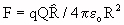 (Equation 3.12)
A graphical representation of this vector E-field is shown in Figure 3.8(a). The direction of the arrows shows the direction of the E-field, and the spacing between the field lines shows the intensity of the field. The field is most intense when the spacing of the field lines is the closest. (See Section 3.1.3 for a discussion of vector-field representations.) Thus near the charge, where the field lines
are close together, the field is strong; and it dies away as the reciprocal of the distance squared from the charge, as
indicated by Equation 3.12. The E-field produced by an infinitely long, uniform line of positive charge is shown in
Figure 3.8(b). In this case the field dies away as the reciprocal of the distance from the line charge. Note that,
in every case, the direction of the E-field line is the direction of the force that would be exerted on a small
positive test charge, q, placed at that point in the field. For a negative point charge, the E-field lines would point toward the charge, since a positive test charge would be attracted toward the negative charge producing the field.
Figure 3.8.
(a) E-field produced by one point charge, Q, in space.
(b)E-field produced by a uniform line of charge (looking down at the top of the line charge).
The sources of static E-fields are charges. For example, E-fields can be produced by charges picked up by a person walking across a deep pile rug. This kind of E-field sometimes produces an unpleasant shock when the person touches a grounded object, such as a water faucet. The charge configurations that produce E-fields are often mechanical devices (such as electric generators) or electrochemical devices (such as automobile batteries).
Figure 3.9 depicts E-field lines between a pair of parallel infinite plates. This field could be produced by connecting a voltage source across the plates, which would charge one plate with positive charge and the other plate with negative charge.
Figure 3.9.
Field lines between infinite parallel conducting plates. Solid lines are E-field lines. Dashed lines are equipotential surfaces.
An important characteristic of E-fields is illustrated in Figure 3.10(a); a small metallic object is
placed in the field between the parallel plates of Figure 3.9. The sharp corners of the object concentrate the E-field, as indicated by the crowding of the field lines around the corners.
Figure 3.10(b) shows how the edges of finite plates also concentrate the field lines. Generally, any sharp object will tend to concentrate the E-field lines. This explains why arcs often occur at corners or sharp points in
high-voltage devices. Rounding sharp edges and corners will often prevent such arcs. Another important principle is that static E-field lines must always be perpendicular to surfaces with high ohmic conductivity. An approximate sketch of E-field lines can often be made on the basis of this principle. For example, consider the field plot in Figure 3.10(a). This sketch can be made by noting that the originally evenly spaced field lines of Figure 3.9 must be modified so that they will be normal to the surface of the metallic object placed between the plates, and they must also be normal to the plates. This concept is often sufficient to understand qualitatively the E-field behavior for a given configuration.
Figure 3.10
(a) E-field lines when a small metallic object is placed between the plates.
(b) E-field lines between parallel conducting plates of finite size.
Figure 3.11. B-field produced by an infinitely long, straight dc element out of the paper.
Static Magnetic Fields--Perhaps the simplest example of a static B-field is that produced by an infinitely long, straight dc element, as shown in Figure 3.11. The field lines circle around the current, and the field dies away as the reciprocal of the distance from the current.
Figure 3.12 shows another example, the B-field produced by a simple circular loop of current. A simple qualitative rule for sketching static B-field lines is that the field lines circle around the current element and are strongest near the current. The direction of the field lines with respect to the direction of the current is obtained from the right-hand rule: Put the thumb in the direction of the positive current and the fingers will circle in the direction of the field lines.
Figure 3.12.
B-field produced by a circular current loop.
An important class of electromagnetic fields is
quasi-static fields. These fields have the same spatial patterns as static fields but vary with time. For example, if
the charges that produce the E-fields in Figures 3.8-3.10 were to vary slowly with time, the field patterns
would vary correspondingly with time but at any one instant would be similar to the static-field patterns shown in the figures. Similar statements could be made for the static B-fields shown in Figures 3.11 and 3.12. Thus when the frequency of the source charges or currents is low enough, the fields produced by the sources can be considered quasi-static fields; the field patterns will be the same as the static-field patterns but will change with time. Analysis of quasi-static fields is thus much easier than analysis of fields that change more rapidly with time, as explained in Section 3.2.7.
Because of the force exerted by an electric field on a charge placed in that field, the charge possesses potential energy. If a charge were placed in an E-field and released, its potential energy would be changed to kinetic energy as the force exerted by the E-field on the charge caused it to move. Moving a charge from one point to another in an E-field requires work by whatever moves the charge. This work is equivalent to the change in potential energy of the charge. The potential energy of a charge divided by the magnitude of the charge is called electric-field potential. E-field potential is a scalar field (see Section 3.1.3). This potential scalar field is illustrated in Figure 3.13 for two cases:
- Fields produced by a point charge
- Fields between two infinite parallel conducting plates
The equipotential surfaces for (a) are spheres; those for (b) are planes. The static E-field lines are always perpendicular to the equipotential surfaces.
For static and quasi-static fields, the difference in E-field potential is the familiar potential difference
(commonly called voltage) between two points, which is used extensively in electric-circuit theory. The difference of potential between two points in an E-field is illustrated in Figure 3.13.
Figure 3.13.
Potential scalar fields (a) for a point charge and (b) between infinite parallel conducting plates. Solid lines are E-field lines; dashed lines are equipotential surfaces.
In each case the potential difference of point P2 with respect to point P1 is positive: Work must be done against the E-field to move a test charge from P1 to P2 because the force exerted on a positive charge by the E-field would be in the general direction from P2 to P1. In
Figure 3.13(b) the E-field between the plates could be produced by charge on the plates transferred by a dc source, such as a battery connected between the plates. In this case the difference in potential of one plate with respect to the other would be the same as the voltage of the battery. This potential difference would be equal to the work required to move a unit charge from one plate to the other.
The concepts of potential difference (voltage) and current are very useful at the lower frequencies, but at
higher frequencies (for example, microwave frequencies) these concepts are not useful and electromagnetic-field theory must be used. More is said about this in Section 3.2.7,
Electric and magnetic fields interact with materials in two ways. First, The E- and B-fields exert forces on the
charged particles in the materials, thus altering the charge pattern that originally existed. Second, the altered charge patterns in the materials produce additional E- and B-fields (in addition to the fields that were originally applied). Materials are usually classified as being either magnetic or nonmagnetic. Magnetic materials have magnetic dipoles that are strongly affected by applied fields; nonmagnetic materials do not.
Nonmagnetic Materials--In nonmagnetic materials, mainly the applied E-field has an effect on the charges in the material. This occurs in three primary ways:
- Polarization of bound charges
- Orientation of permanent dipoles
- Drift of conduction charges (both electronic and ionic)
Materials primarily affected by the first two kinds are called dielectrics; materials primarily affected by the third
kind, conductors.
The polarization of bound charges is illustrated in Figure 3.14 (a ). Bound charges are so tightly bound by restoring forces in a material that they can move only very slightly. Without an applied E-field, positive and negative bound charges in an atom or molecule are essentially superimposed upon each other and effectively cancel out; but when an E-field is applied, the forces on the positive and negative charges are in opposite directions and the charges separate, resulting in an induced electric dipole. A dipole consists of a combination of a positive and a negative charge separated by a small distance. In this case the dipole is said to be induced because it is caused by the applied E-field; when the field is removed, the dipole disappears. When the charges are separated by the applied E-field, the
charges no longer cancel; in effect a new charge is created, called polarization charge, which creates new fields that did not exist previously.
The orientation of permanent dipoles is illustrated in Figure 3.14(b). The arrangement of charges in some molecules produces permanent dipoles that exist whether or not an E-field is applied to the material. With no E-field applied, the permanent dipoles are randomly oriented because of thermal excitation. With an E-field applied, the resulting forces on the permanent dipoles tend to align the dipole with the applied
E-field (Figure 3.14(b)).
Figure 3.14.
(a) Polarization of bound charges. (b) Orientation of permanent dipoles.
The orientation of each dipole is slight because the thermal excitation is relatively strong, but on the average
there is a net alignment of dipoles over the randomness that existed without an applied E-field. Like induced dipoles, this net alignment of permanent dipoles produces new fields.
The drift of conduction charges in an applied E-field occurs because these charges are free enough to move significant distances in response to forces of the applied fields. Both electrons and ions can be conduction charges. Movement of the conduction charges is called drift because thermal excitation causes random motion of the conduction charges, and the forces due to the applied fields superimpose only a slight movement in the direction of the forces on this random movement. The drift of conduction charges amounts to a current, and this current produces new fields that did not exist before E-fields were applied.
Permittivity--The two effects--creation of new charges by an applied field and creation of new fields by these new charges--are both taken into account for induced dipoles and orientation of permanent dipoles by a quantity called permittivity. Permittivity is a measure of how easily the polarization in a material occurs. If an applied
E-field results in many induced dipoles per unit volume or a high net alignment of permanent dipoles per unit volume, the permittivity is high. The drift of conduction charges is accounted for by a quantity called conductivity. Conductivity is a measure of how much drift occurs for a given applied E-field. A large drift means a high conductivity. For sinusoidal steady-state applied fields, complex permittivity is defined to account for both dipole charges and conduction-charge drift. Complex permittivity is usually designated as
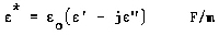 (Equation 3.13)
where  o is the permittivity of free space; ' - j", the complex relative permittivity; ', the real part of the complex relative permittivity (' is also called the dielectric constant); and ", the imaginary part of the complex relative permittivity. This notation is used when the time variation of the electromagnetic fields is described by ejwt, where j =
  and
and  is the radian frequency. Another common practice is to describe the time variation of the fields by e-iwt, where i =. For this case complex permittivity is defined by * = o (' + i"). " is related to the effective conductivity by
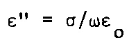 (Equation 3.14)
where  is the effective conductivity, o is the permittivity of free space, and
 (Equation 3.15)
is the radian frequency of the applied fields. The ' of a material is primarily a measure of the relative
amount of polarization that occurs for a given applied E-field, and the " is a measure of both the
friction associated with changing polarization and the drift of conduction charges.
Generally is used to designate permittivity; * is usually used only for sinusoidal steady-state fields.
Energy Absorption--Energy transferred from applied E-fields to materials is in the form of kinetic energy of the charged particles in the material. The rate of change of the energy transferred to the material is the power transferred to the material. This power is often called absorbed power, but the bioelectromagnetics community has accepted specific absorption rate (SAR) as a preferred term (see Section 3.3.6).
A typical manifestation of average (with respect to time) absorbed power is heat. The average absorbed power results from the friction associated with movement of induced dipoles, the permanent dipoles, and the drifting conduction charges. If there were no friction in the material, the average power absorbed would be zero.
A material that absorbs a significant amount of power for a given applied field is said to be a lossy material because of the loss of energy from the applied fields. A measure of the lossiness of a material is ": The larger the ", the more lossy the material. In some tables a quantity called the loss tangent is listed instead of ". The loss tangent, often designated as tan  , is defined as
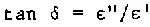 (Equation 3.16)
The loss tangent usually varies with frequency. For example, the loss tangent of distilled water is about 0.040
at 1 MHz and 0.2650 at 25 GHz. Sometimes the loss factor is called the dissipation factor. Generally speaking, the wetter a material is, the more lossy it is; and the drier it is, the less lossy it is. For example, in a microwave oven a wet piece of paper will get hot as long as it is wet; but when the paper dries out, it will no longer be heated by the oven's electromagnetic fields.
For steady-state sinusoidal fields, the time-averaged power absorbed per unit volume at a point inside an absorber is given by
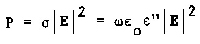 (Equation 3.17)
where |E| is the root-mean-square (rms) magnitude of the E-field vector at that point inside the
material. If the peak value of the E-field vector is used, a factor of 1/2 must be included on the right-hand side of
Equation 3.17.' The rms and peak values are explained in Section 3.2.8. Unless otherwise noted, rms values are usually given. To find the total power absorbed by an object, the power density given by Equation 3.17 must be calculated at each point inside the body and summed (integrated) over the entire volume of the body. This is usually a very complicated calculation.
Electric-Flux Density--A quantity called electric-flux density or displacement-flux-density is defined as
 (Equation 3.18)
An important property of D is that its integral over any closed surface (that is, the total flux passing through the closed surface) is equal to the total free charge (not including polarization or conduction charge in materials)
inside the closed surface. This relationship is called Gauss's law. Figure 3.15 shows an example of this. The total flux passing out through the closed mathematical surface, S, is equal to the total charge, Q, inside S, regardless of what the permittivity of the spherical shell is. Electric-flux density is a convenient quantity because it is independent of the charges in materials.
Figure 3.15.
Charge Q inside a dielectric spherical shell. S is a closed mathematical surface.
Magnetic Materials--Magnetic materials have magnetic dipoles that tend to be oriented by applied magnetic fields. The resulting motion of the magnetic dipoles produces a current that creates new E- and B-fields. Both the effect of the applied fields on the material and the creation of new fields by the moving magnetic dipoles in the material are accounted for by a property of the material called permeability.
For sinusoidal steady-state fields, the complex permeability is usually designated as
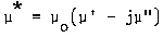 (Equation 3.19)
where  ' - j" is the complex relative permeability and o is the permeability of free space. For the general case, permeability is usually designated by .
Another field quantity, H, or magnetic field intensity, is defined by
 (Equation 3.20)
The magnetic-field intensity is a useful quantity because it is independent of magnetic currents in materials. The term "magnetic field" is often applied to both B and H. Whether to use B or H in a given situation is not always clear, but since they are related by Equation 3.20, either could usually be specified.
Since biological materials are mostly nonmagnetic, permeability is usually not an important factor in
bioelectromagnetic interactions.
Four equations, along with some auxiliary relations, form the theoretical foundation for all classical
electromagnetic-field theory. These are called Maxwell's equations, named for James Clerk Maxwell, the famous Scotsman who added a missing link to the electromagnetic-field laws known at that time and formulated them in a unified form. These equations are very powerful, but they are also complicated and difficult to solve. Although mathematical treatment of these equations is beyond the stated scope of this document, for background information we will list the equations and describe them qualitatively. Maxwell's equations for fields are
 (Equation 3.21)
 (Equation 3.22)
 (Equation 3.23)
 (Equation 3.24)
where
B =H
D =E
J is free-current density in A/m 2
 is free-charge density in C/m 3
 x stands for a mathematical operation involving partial derivatives, called the curl
· stands for another mathematical operation involving partial derivatives,
called the divergence
x stands for a mathematical operation involving partial derivatives, called the curl
· stands for another mathematical operation involving partial derivatives,
called the divergence
 B/t andD/t are the time rate of change of B and D respectively.
The other quantities have been defined previously.
Any vector field can be completely defined by specifying both the curl and the divergence of the field. Thus the quantities equal to the curl and the divergence of a field are called sources of the field. The terms on the right-hand side of Equations 3.21 and 3.22 are sources related to the curl of the fields on the left-hand side, and the terms on the right-hand side of Equations 3.23 and 3.24 are sources related to the divergence of the fields on the left-hand side.
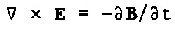
Equation 3.21 thus means that a time-varying B-field produces an E-field, and the
relationship is such that the E-field lines so produced tend to encircle the B-field lines. Equation
3.21 is called Faraday's law.
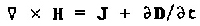
Equation 3.22 states that both current density and a time-varying E-field produce a B-field. The B-field lines so produced tend to encircle the current density and the E-field lines. Since a time-varying E-field acts like current density in producing a B-field, the last term on the right in Equation 3.22 is called displacement current density.
Equation 3.23 states that charge density produces an E-field, and the E-field lines produced by the charges begin and end on those charges.
Equation 3.24 states that no sources are related to the divergence of the B-field. This means that the B-field lines always exist in closed loops; there is nothing analogous to electric charge for the B-field lines either to begin or end on.
Equations 3.21 and 3.22 show that the E- and B-fields are coupled together in the time-varying case because a changing B is a source of E in Equation 3.21 and a changing D is a source of H in Equation 3.22. For static fields, however, B/ t = 0 and D/ t = 0 and the E- and B-fields are not coupled together; thus the static equations are easier to solve.
Since Maxwell's equations are generally difficult to solve, special techniques have been developed to solve them within certain ranges of parameters . One class of solutions, electromagnetic waves, is discussed next. Techniques useful for specific frequency ranges are discussed in Section 3.2.9.

Go to Chapter 3.2.8
Return to Table of Contents.
Last modified: June 14, 1997
© October 1986, USAF School of Aerospace Medicine, Aerospace Medical Division (AFSC), Brooks Air Force Base, TX 78235-5301
(Equation 3.6)