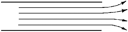
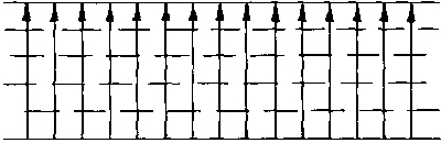
3.9. Field lines between infinite parallel conducting plates

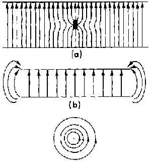
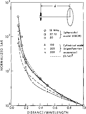
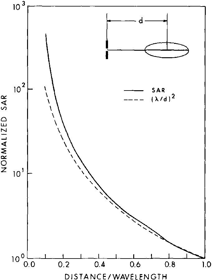
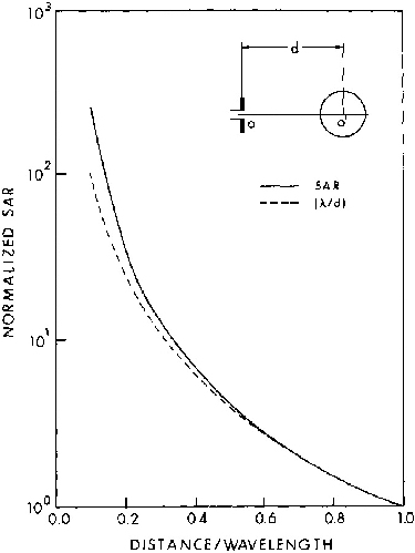
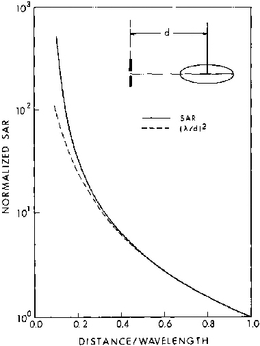
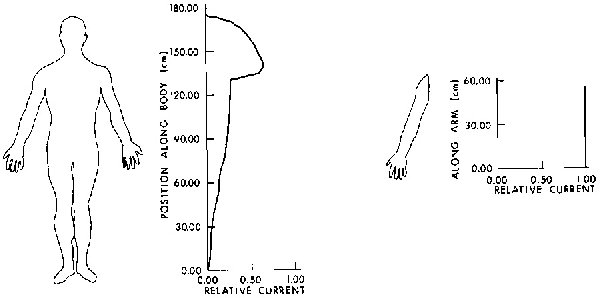
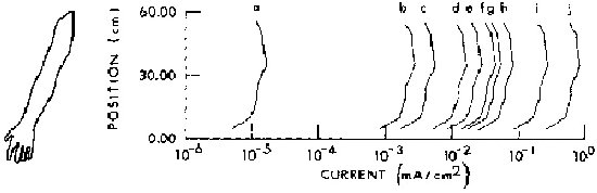
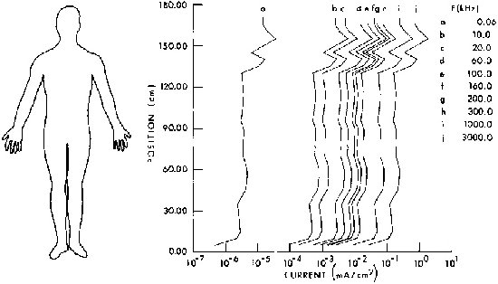
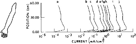
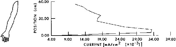
3.10. (a) E-field lines when a small metallic object is placed between the plates

3.11. B-field produced by an infinitely long, straight dc element out of the paper

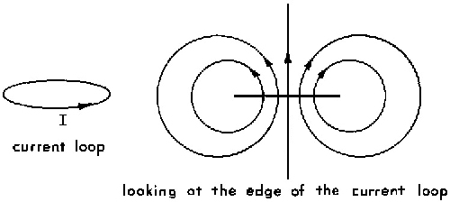
3.12. B-field produced by a circular current loop

3.13. Potential scalar fields (a) for a point charge and (b) between infinite parallel conducting plates

3.14. (a) Polarization of bound charges (b) Orientation of permanent dipoles

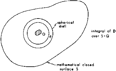
3.15. Charge Q inside a dielectric spherical shell

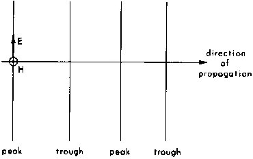
3.16. Snapshots of a traveling wave at two instants of time

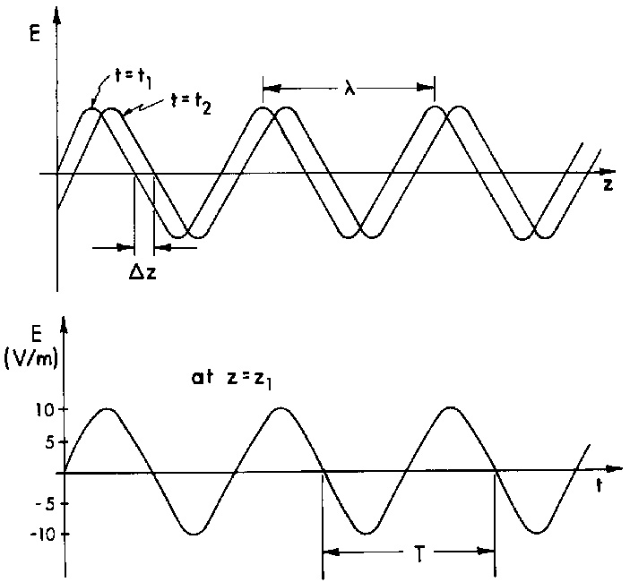
3.17. The variation of E at one point in space as a function of time

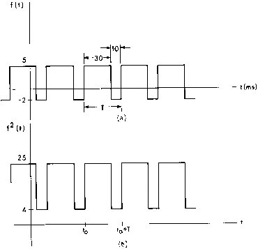
3.18. (a) A given periodic function versus time (b) The square of the function versus time

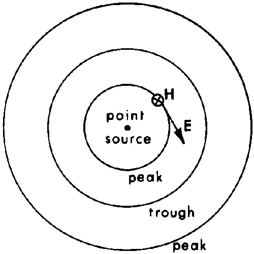
3.19. A spherical wave

3.20. A planewave

3.21. Cross-sectional views of the electric- and magnetic-field lines in the TEM mode for coaxial cable and twin lead

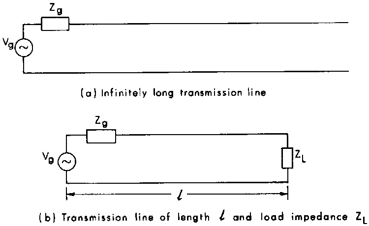
3.22. Schematic diagrams of two-conductor transmission lines

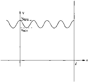
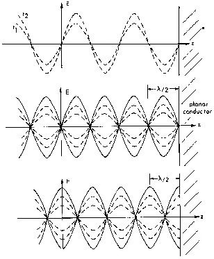
3.23. Total waves, incident plus reflected

3.24. Top half of the envelope resulting from an incident and reflected voltage wave

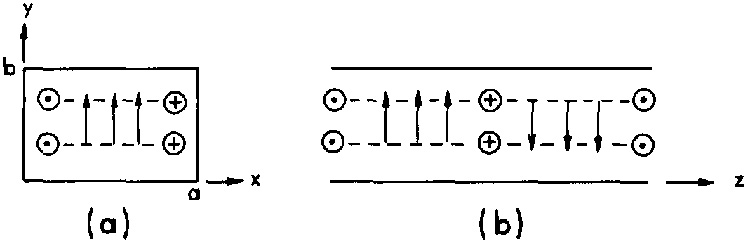
3.25. Field variation of the TE₁₀ mode in a rectangular waveguide

3.26. Some relative cutoff frequencies for a waveguide with b = a/2, normalized to that of the TE₁₀ mode

3.27. A volume bounded by a closed surface

3.28. A planewave irradiating an absorber

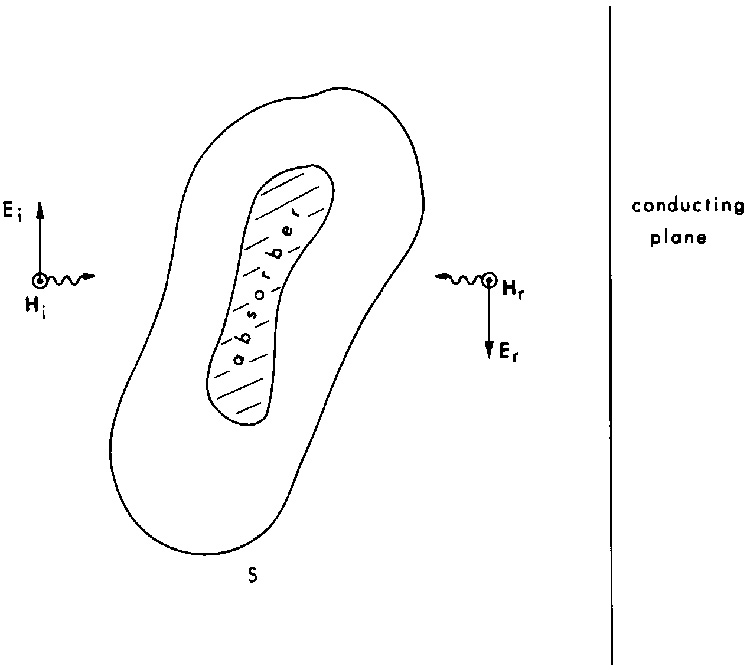
3.29. Absorber placed between an incident planewave and a conducting plane

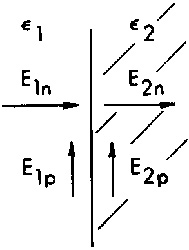
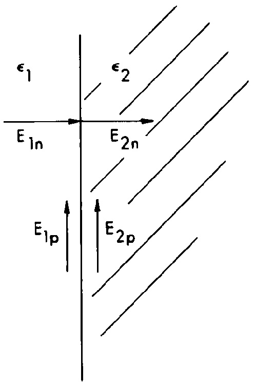
3.30. Electric-field components at a boundary between two materials

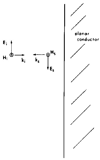
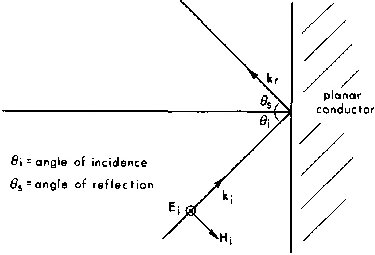
3.31. Planewave incident on a planar conductor

3.32. Total fields, incident plus scattered

3.33. Planewave obliquely incident on a planar conductor

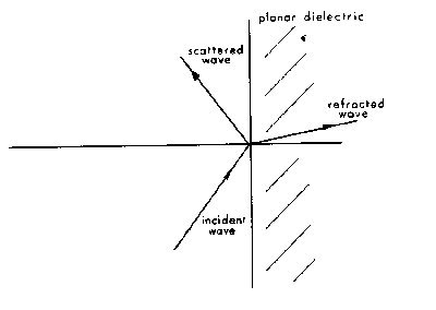
3.34. Planewave obliquely incident on a planar dielectric

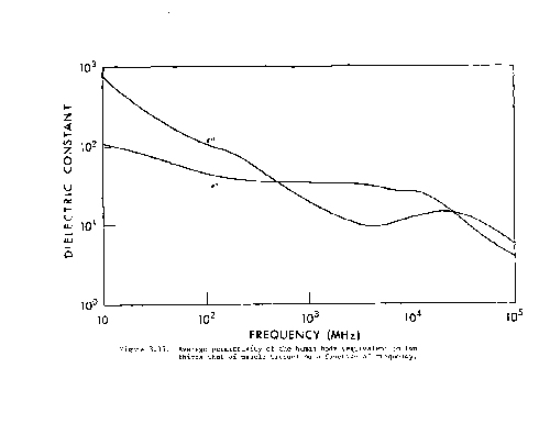
3.35. Average permittivity of the human body (equivalent to two-thirds that of muscle tissue) as a function of frequency

3.36. Skin depth versus frequency for a dielectric half-space with permittivity equal to two-thirds that of muscle

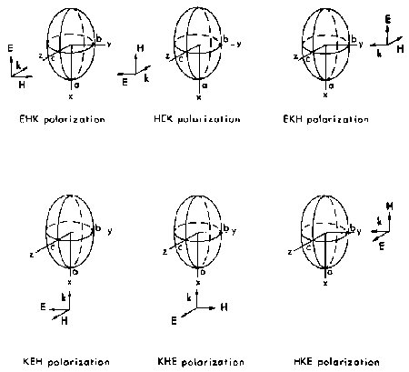
3.37. Polarization of the incident field with respect to an irradiated object

3.38. Polarizations for objects that do not have circular symmetry about the long axis

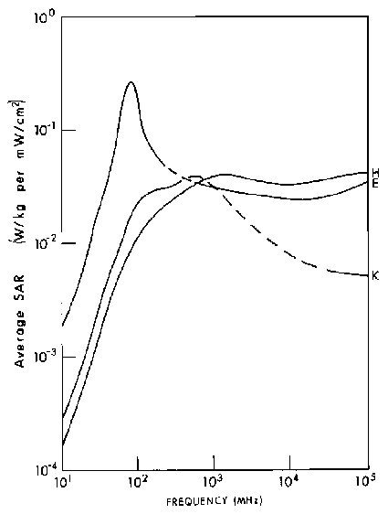
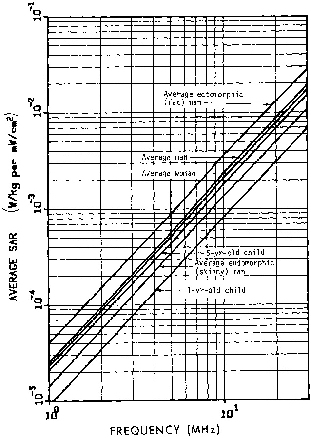
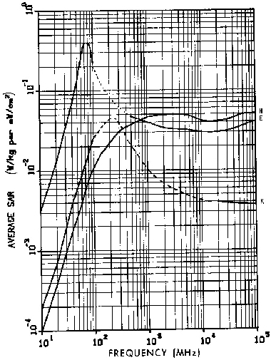
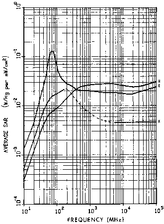
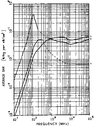
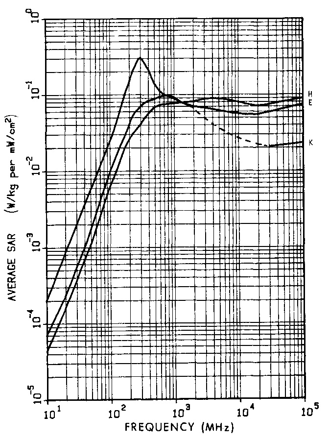
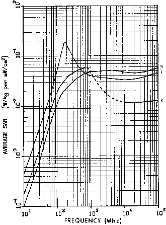
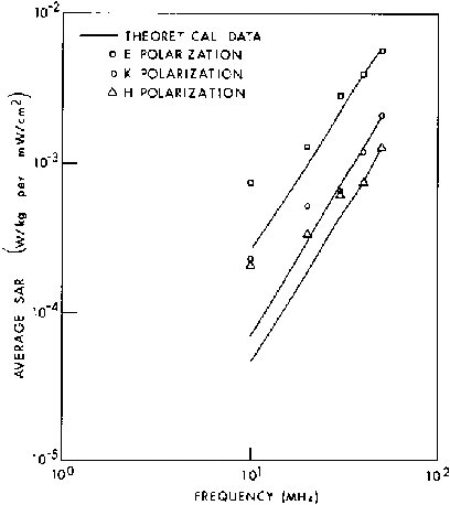
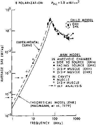
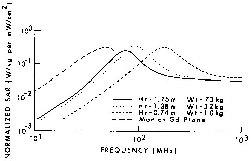
3.39. Calculated whole-body average SAR versus frequency for models of an average man for three standard polarizations

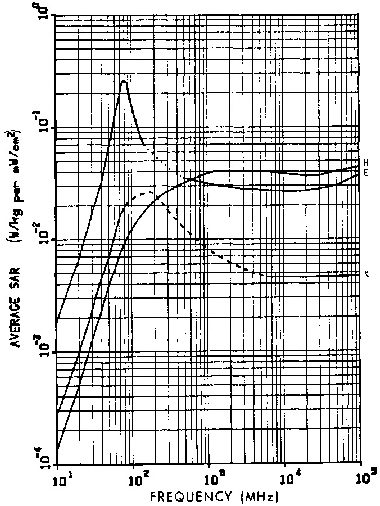
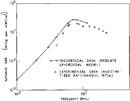
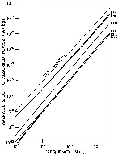
3.40. Calculated whole-body average SAR versus frequency for models of a medium-sized rat, for three standard polarizations

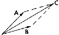
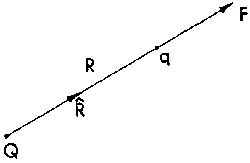
3.41. Short dipole used to sense the presence of an electric field

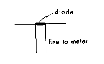
3.42. Simple electric-field probe with a diode detector

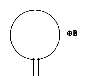
3.43. Loop antenna used as a pickup for measuring magnetic field

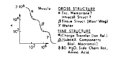
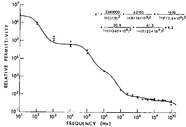
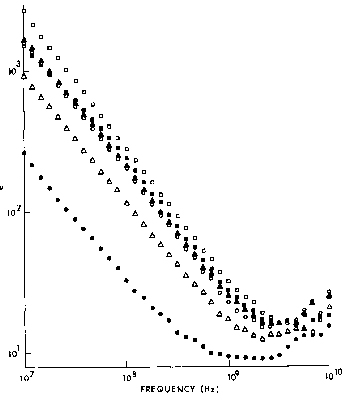
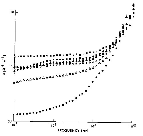
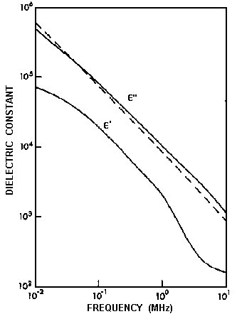
4.1. Frequency dependence of the dielectric constant of muscle tissue

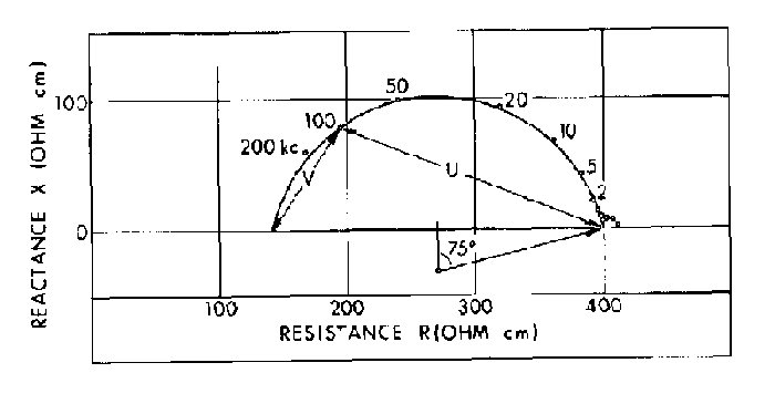
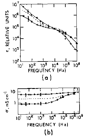
4.2. Dielectric properties of muscle in the impedance plane

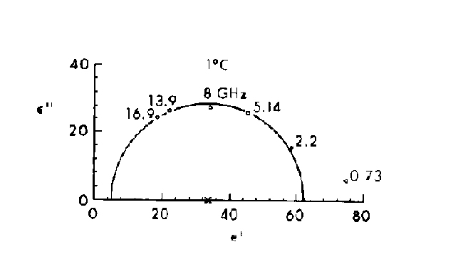
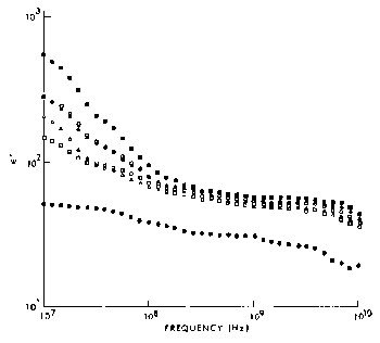
4.3. Dielectric properties of barnacle muscle in the microwave frequency range are presented in the complex dielectric constant plane

4.4. Equivalent circuit for the -dispersion of a cell suspension and corresponding plot in the complex dielectric constant plane

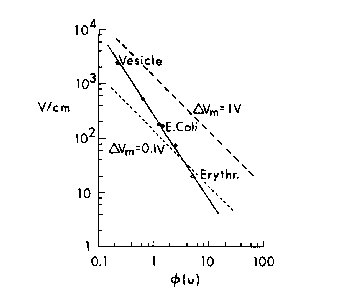
4.5. Threshold field-strength values as a function of particle size

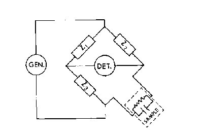
4.6. Bridge circuit for measuring dielectric properties of materials at frequencies below 100 MHz

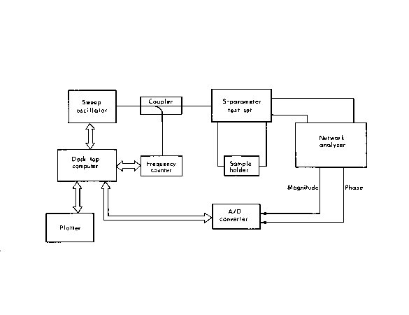
4.7. Experimental setup for measuring S-parameters, using an automatic network analyzer

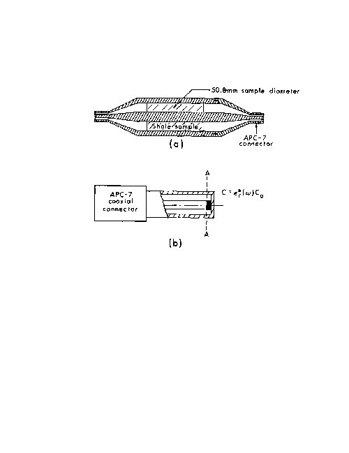
4.8. Typical sample holders for measuring the dielectric properties of biological substances at microwave frequencies

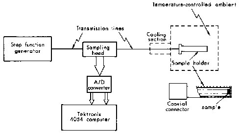
4.9. Typical experimental setup for time-domain measurement of complex permittivities

4.10. In vivo dielectric probes for measuring dielectric properties of biological substances

4.11. Graphical illustration of the iterative procedure for calculating complex permittivity parameters by minimizing the difference between measured and calculated values of the input impedance of the in vivo dielectric probe

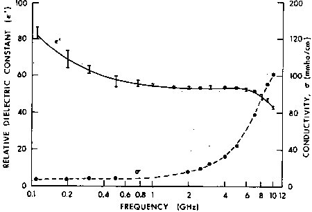
4.12. Relative dielectric permittivity for muscle

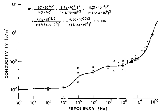
4.13. Conductivity for muscle

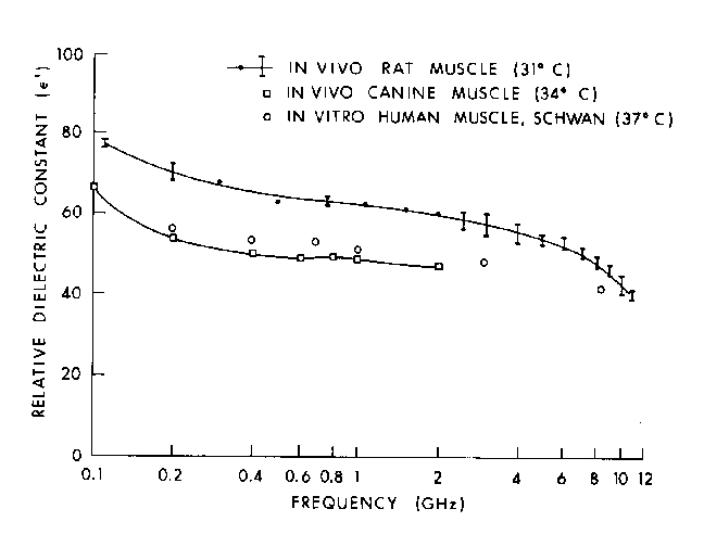
4.14. Measured values of relative dielectric constant of in vivo rat muscle and canine muscle compared to reference data

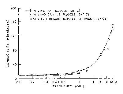
4.15. Measured values of conductivity of in vivo rat muscle and canine muscle compared to reference data

4.16. Measured values of relative dielectric constant and conductivity of in vivo and in vitro canine kidney cortex compared to reference data

4.17. Measured values of relative dielectric constant and conductivity of in vivo canine fat tissue at 37° C

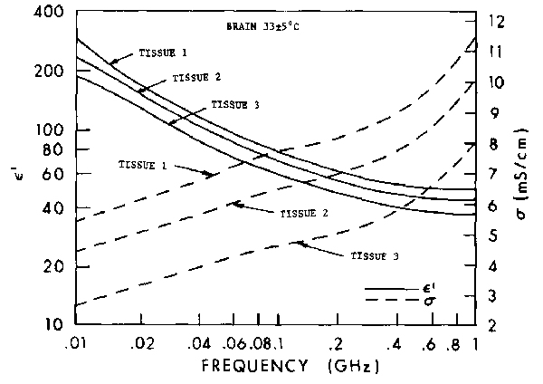
4.18. Measured values of relative dielectric constant and conductivity of in vivo rat brain at 32° C

4.19. Measured values of relative dielectric constant and conductivity of rat blood at 23° C

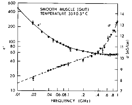
4.20. Relative permittivity of cat smooth muscle in vivo

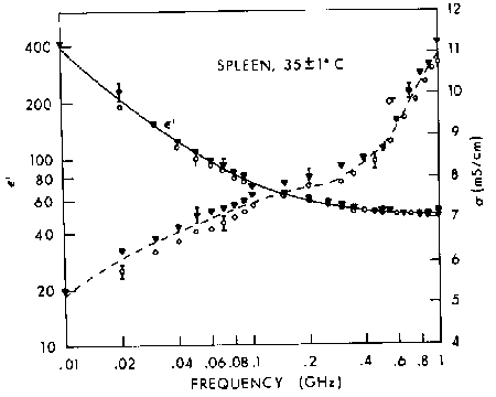
4.21. Relative permittivity of cat spleen in vivo

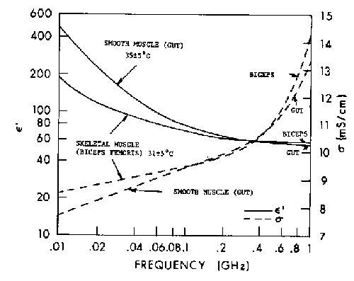
4.22. Average relative permittivity of two types of cat muscle in vivo

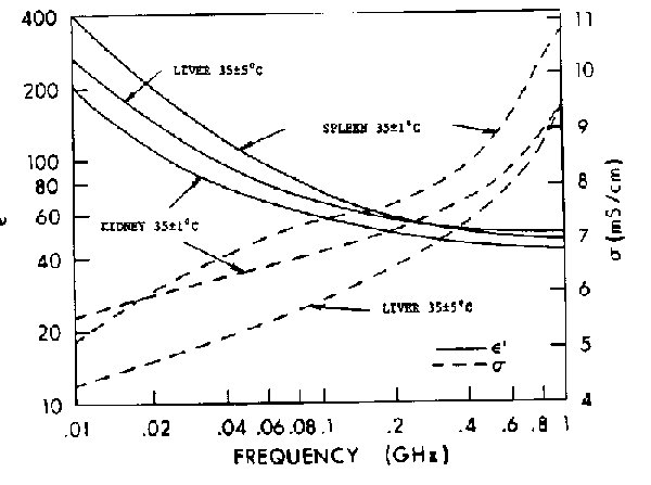
4.23. Average relative permittivity of cat internal organs in vivo

4.24. Relative permittivity of cat brain tissue

4.25. The real part of the dielectric constant and conductivity of the canine skeletal muscle tissue at 37° C as a function of frequency, in parallel orientation and perpendicular orientation, averaged over five measurements on different samples

4.26. The real part of the dielectric constant of ocular tissues at 37° C

4.27. The imaginary part of the dielectric constant of ocular tissues at 37° C

4.28. The conductivity of ocular tissues at 37° C

4.29. The real part of the dielectric constant of normal and tumor mouse tissue as a function of frequency

4.30. Conductivity of normal and tumor mouse tissue as a function of frequency

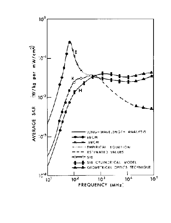
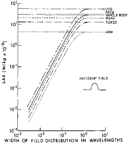
5.1. Illustration of different techniques, with their frequency limits, used for calculating SAR data for models of an average man

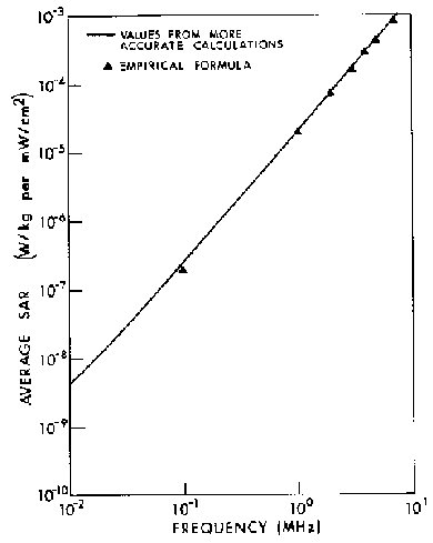
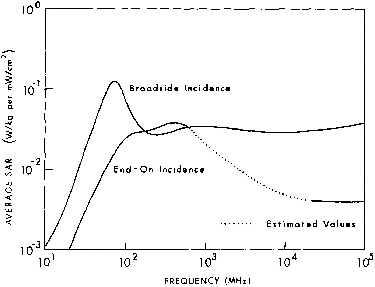
5.2. Average SAR calculated by the empirical formula compared with the curve obtained by other calculations for a 70-kg man in E polarization

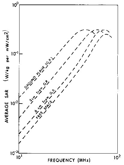
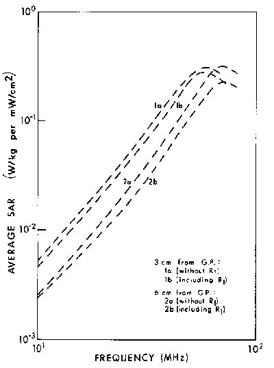
5.3. Calculated effect of a capacitive gap, between man model and ground plane, on average SAR

5.4. Calculated effect of grounding resistance on SAR of man model placed at a distance from ground plane

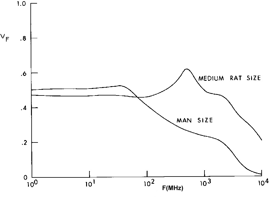
5.5. The volume fraction as a function of frequency for a cylindrical model of an average man

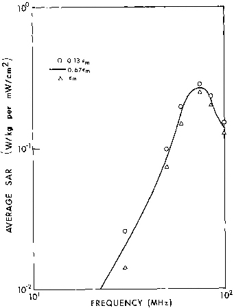
5.6. The volume fraction as a function of frequency for two spheres of muscle material

5.7. Calculated average SAR in a prolate spheroidal model of an average man, as a function of frequency for several values of permittivity

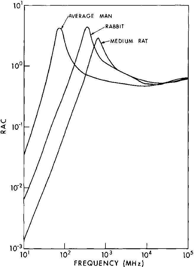
5.8. Relative absorption cross section in prolate spheroidal models of an average man, a rabbit, and a medium-sized rat--as a function of frequency for E polarization

5.9. Comparison of relative scattering cross section and relative absorption cross section in a prolate spheroidal model of a medium rat--for planewave irradiation, E polarization

5.10. Field components at a boundary between two media having different complex permittivities

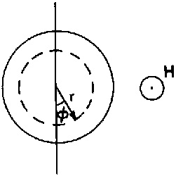
5.11. A lossy dielectric cylinder in a uniform magnetic field

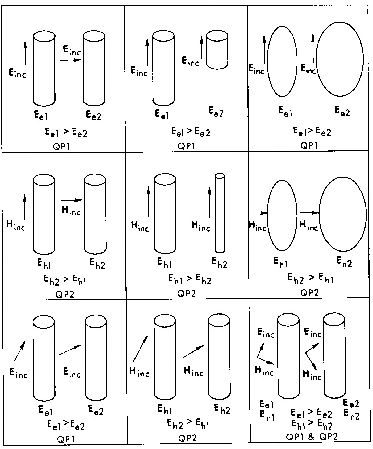
5.12. Qualitative evaluation of the internal fields based on qualitative principles QPI and QP2

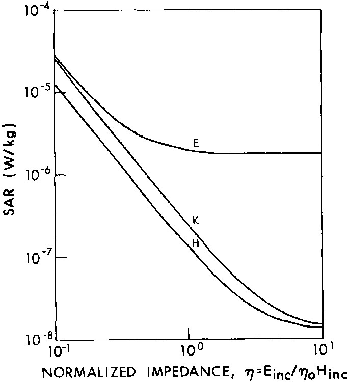
5.13. Average SAR in a prolate spheroidal model of an average man as a function of normalized impedance for each of three polarizations

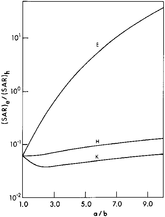
5.14. Ratio of (SAR)_e to (SAR)_h of a 0.07-m³ prolate spheroid for each polarization as a function of the ratio of the major axis to the minor axis of the spheroid at 27.12 MHz

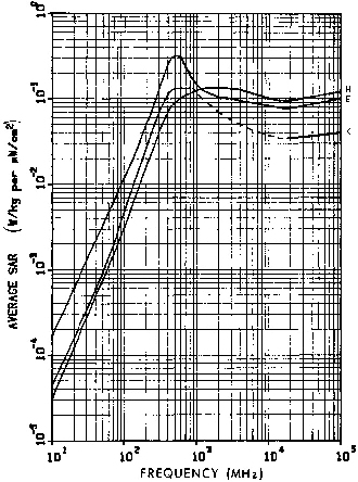
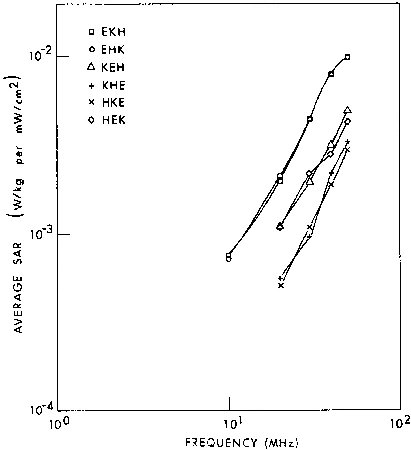
6.1. Calculated planewave average SAR in an ellipsoidal model of an average man, for the six standard polarizations

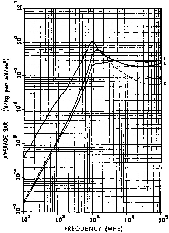
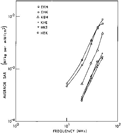
6.2. Calculated planewave average SAR in ellipsoidal models of different human-body types, EKH polarization

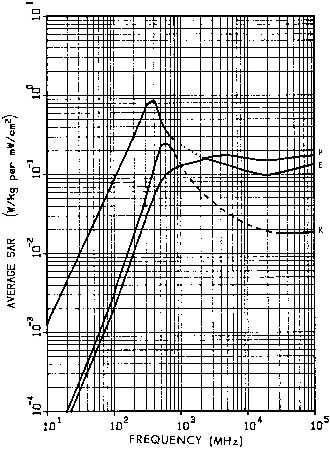
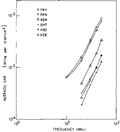
6.3. Calculated planewave average SAR in a prolate spheroidal model of an average man for three polarizations

6.4. Calculated planewave average SAR in a prolate spheroidal model of an average ectomorphic (skinny) man for three polarizations

6.5. Calculated planewave average SAR in a prolate spheroidal model of an average endomorphic (fat) man for three polarizations

6.6. Calculated planewave average SAR in a prolate spheroidal model of an average woman for three polarizations

6.7. Calculated planewave average SAR in a prolate spheroidal model of a large woman for three polarizations

6.8. Calculated planewave average SAR in a prolate spheroidal model of a 5-year-old child for three polarizations

6.9. Calculated planewave average SAR in a prolate spheroidal model of a 1-year-old child for three polarizations

6.10. Calculated planewave average SAR in a prolate spheroidal model of a sitting rhesus monkey for three polarizations

6.11. Calculated planewave average SAR in a prolate spheroidal model of a squirrel monkey for three polarizations

6.12. Calculated planewave average SAR in a prolate spheroidal model of a Brittany spaniel for three polarizations

6.13. Calculated planewave average SAR in a prolate spheroidal model of a rabbit for three polarizations

6.14. Calculated planewave average SAR in a prolate spheroidal model of a guinea pig for three polarizations

6.15. Calculated planewave average SAR in a prolate spheroidal model of a small rat for three polarizations

6.16. Calculated planewave average SAR in a prolate spheroidal model of a medium rat for three polarizations

6.17. Calculated planewave average SAR in a prolate spheroidal model of a large rat for three polarizations

6.18. Calculated planewave average SAR in a prolate spheroidal model of a medium mouse for three polarizations

6.19. Calculated planewave average SAR in a prolate spheroidal model of a quail egg for three polarizations

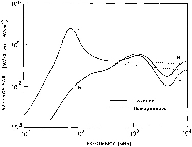
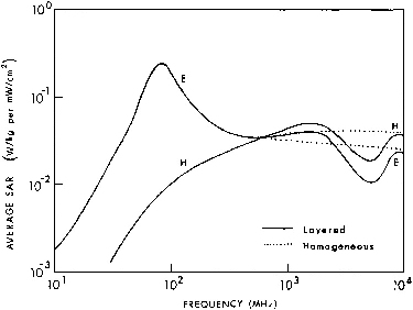
6.20. Calculated planewave average SAR in homogeneous and multilayered models of an average man for two polarizations

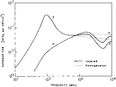
6.21. Calculated planewave average SAR in homogeneous and multilayered models of an average woman for two polarizations

6.22. Calculated planewave average SAR in homogeneous and multilayered models of a 10-year-old child for two polarizations

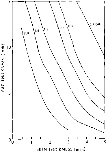
6.23. Layering resonance frequency as a function of skin and fat thickness for a skin-fat-muscle cylindrical model of man, planewave H polarization

6.24. Layering resonance frequency as a function of skin and fat thickness for a skin-fat-muscle cylindrical model of man, planewave E polarization

6.25. Calculated planewave average SAR in a prolate spheroidal model of an average man irradiated by a circularly polarized wave, for two orientations

6.26. Calculated planewave average SAR in a prolate spheroidal model of a sitting rhesus monkey irradiated by a circularly polarized wave, for two orientations

6.27. Calculated planewave average SAR in a prolate spheroidal model of a medium rat irradiated by a circularly polarized wave, for two orientations

6.28. Calculated planewave average SAR in a prolate spheroidal model of an average man irradiated by an elliptically polarized wave, for two orientations

6.29. Calculated planewave average SAR in a prolate spheroidal model of a sitting rhesus monkey irradiated by an elliptically polarized wave, for two orientations

6.30. Calculated planewave average SAR in a prolate spheroidal model of a medium rat irradiated by an elliptically polarized wave, for two orientations

6.31. Calculated normalized average SAR as a function of the electric dipole location for E polarization in a prolate spheroidal model of an average man

6.32. Calculated average SAR (by long-wavelength approximation) as a function of the electric dipole location for K polarization at 27.12 MHz in a prolate spheroidal model of an average man

6.33. Calculated average SAR (by long-wavelength approximation) as a function of the electric dipole location for H polarization at 27.12 MHz in a prolate spheroidal model of an average man

6.34. Calculated average SAR (by long-wavelength approximation) as a function of the electric dipole location for E polarization at 100 MHz in a prolate spheroidal model of a medium rat

6.35. Calculated average SAR (by long-wavelength approximation) as a function of the electric dipole location for K polarization at 100 MHz in a prolate spheroidal model of a medium rat

6.36. Calculated average SAR (by long-wavelength approximation) as a function of the electric dipole location for H polarization at 100 MHz in a prolate spheroidal model of a medium rat

6.37. Calculated normalized E-field of a short electric dipole,as a function of y/ at z = 30 cm

6.38. Calculated normalized H-field of a short electric dipole,as a function of y/ at z = 30 cm

6.39. Calculated variation of a as a function of y/, at z =30 cm, for a short electric dipole

6.40. Calculated normalized field impedance of a short electric dipole, as a function of y/ at z = 30 cm

6.41. Calculated average SAR in a prolate spheroidal model of an average man irradiated by the near fields of a short electric dipole, as a function of the dipole-to-body spacing, d

6.42. Calculated average SAR in a prolate spheroidal model of an average man irradiated by the near fields of a small magnetic dipole, as a function of the dipole-to-body spacing, d

6.43. The block model of man used by Chatterjee et al. (1980a, 1980b, 1980c) in the planewave spectrum analysis

6.44. Incident-field E_z from a 27.12-MHz RF sealer, used by Chatterjee et al. (1980a, 1980b, 1980c) in the planewave angular-spectrum analysis

6.45. Average whole- and part-body SAR in the block model of man placed in front of a half-cycle cosine field, E_z ; frequency = 27.12 MHz, E_z | _max = 1 V/m

6.46. Average whole- and part-body SAR in the block model of man placed in front of a half-cycle cosine field, E_z ; frequency = 77 MHz, E_z | _max = 1 V/m

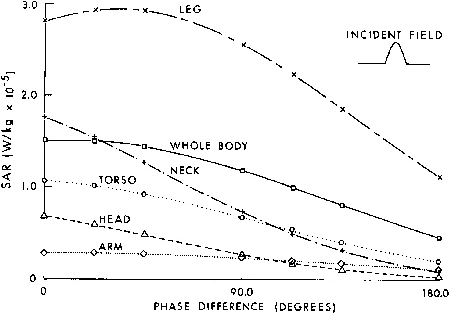
6.47. Whole- and part-body SAR at 77 MHz in the block model of man as a function of an assumed linear antisymmetric phase variation in the incident E_z ; E_z | _max = 1 V/m

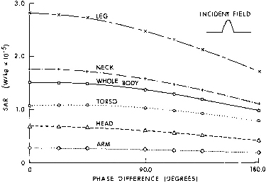
6.48. Whole- and part-body SAR at 77 MHz in the block model of man as a function of an assumed linear symmetric phase variation in the incident E_z ; E_z | _max = 1 V/m

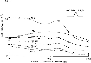
6.49. Whole- and part-body SAR at 350 MHz in the block model of man as a function of an assumed linear antisymmetric phase variation in the incident E_z ; E_z | _max = 1 V/m

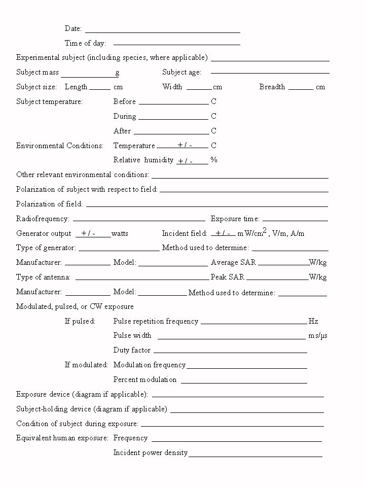
7.1. A data sheet for RFR bioeffects research

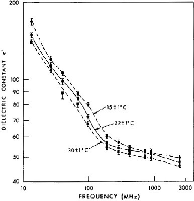
7.2. Relative permittivity of simulated muscle tissue versus frequency for three temperatures

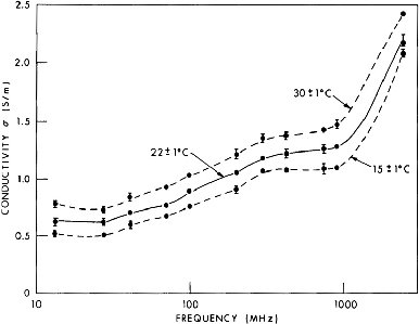
7.3. Electrical conductivity of simulated muscle tissue versus frequency for three temperatures

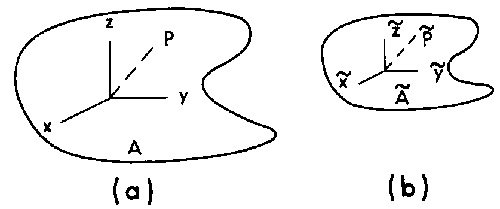
7.4. Schematic diagram illustrating the coordinate system used in the scaling procedure

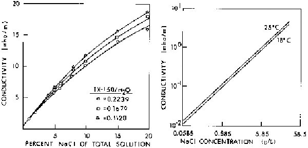
7.5. Electrical conductivity of phantom muscle as a function of NaCl and TX-150 contents measured at 100 kHz and 23° C

7.6. Electrical conductivity of saline solution as a function of the aqueous sodium chloride concentration

7.7. Electrical conductivity of saline solution as a function of the NaCl concentration at 25° C

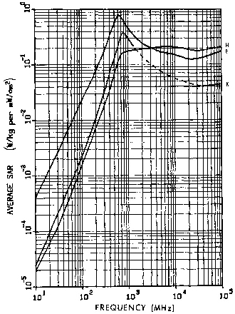
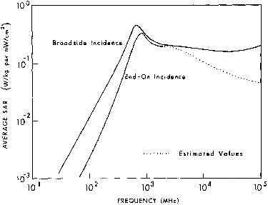
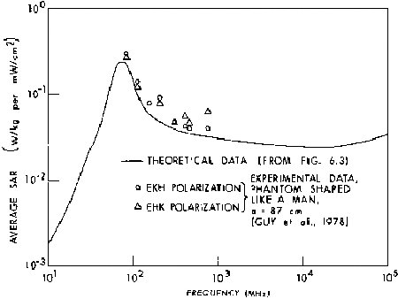
8.1A. Comparison of measured (experimental) and calculated (theoretical) SAR values for an average man in free space, E polarization

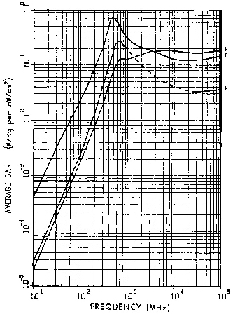
8.2B. Comparison of measured and calculated SAR values for an average man in free space, H and K polarizations

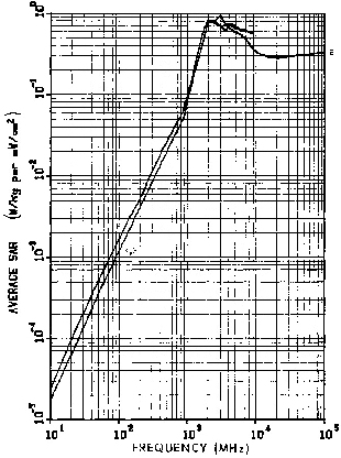
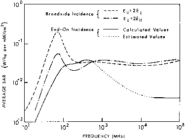
8.2. Calculated and measured values of the average SAR for a human prolate spheroidal phantom

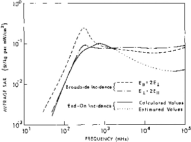
8.3. Calculated and measured values of the average SAR for a prolate spheroidal phantom of a sitting rhesus monkey

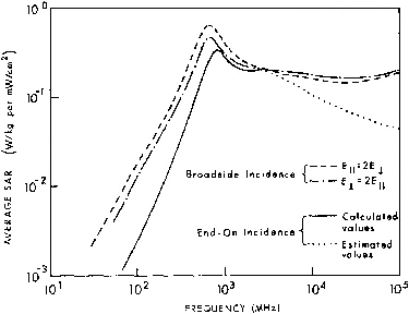
8.4. Measured values of the average SAR for a live, sitting rhesus monkey, for six standard polarizations

8.5. Measured values of the average SAR for saline-filled ellipsoidal phantoms, for six standard polarizations; a = 20 cm, b = 7.92 cm, c = 5.28 cm, = 0.64 S/m

8.6. Measured values of the average SAR for saline-filled ellipsoidal phantoms, for six standard polarizations; a = 20 cm, b = 7.92 cm, c = 5.28 cm, = 0.54 S/m

8.7. Measured values of the average SAR for saline-filled ellipsoidal phantoms, for six standard polarizations; a = 20 cm, b = 7.92 cm, c = 5.28 cm, = 0.36 s/m

8.8. Calculated and measured values of the average SAR for models of an average man, E polarization

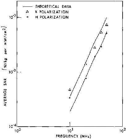
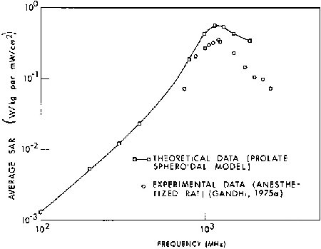
8.9. Calculated and measured values of the average SAR for a 96-g rat, K polarization

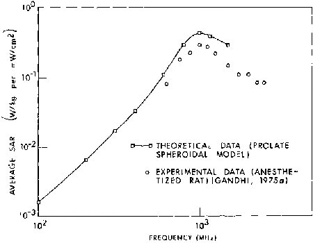
8.10. Calculated and measured values of the average SAR for a 158-g rat, K polarization

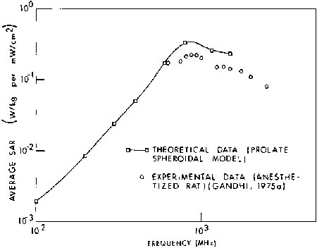
8.11. Calculated and measured values of the average SAR for a 261-g rat, K polarization

8.12. Calculated and measured values of the average SAR for a 390-g rat, K polarization

8.13. Calculated and measured values of the average SAR for models of a rat, H polarization

8.14. Calculated and measured values of the average SAR for models of a rat, K polarization

8.15. Calculated and measured values of the average SAR for models of a rat, E polarization

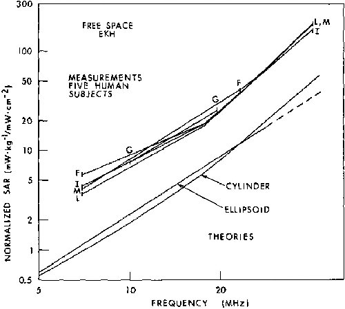
8.16. Comparison of free-space absorption rates of five human subjects with each other and with two standard theories

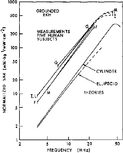
8.17. Comparison of the grounded absorption rates of five human subjects with each other and with two standard theories

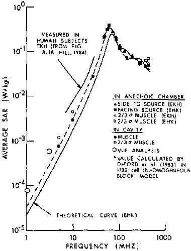
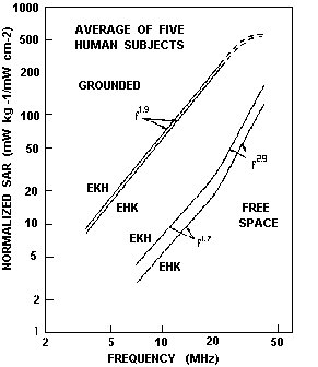
8.18. Frequency dependence of the average absorption rates for five human subjects in the EKH and EHK, orientations under both free-space and grounded conditions

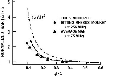
8.19. Measured relative SARs in scaled saline spheroidal models of man

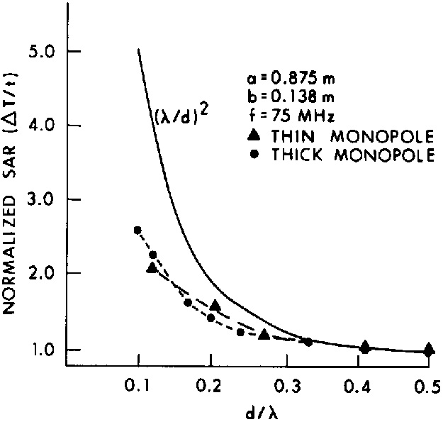
8.20. Measured relative SARs in scaled saline spheroidal models versus distance

8.21. Measured relative fields versus distance for the thick monopole on a grounded plane. The values of E and H are normalized with respect to their values at d/ = 0.6

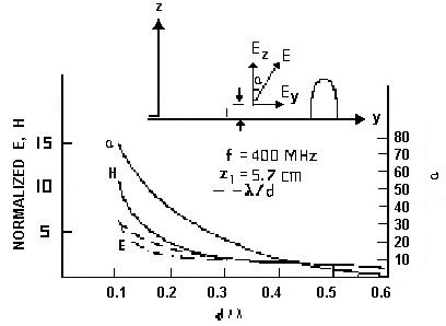
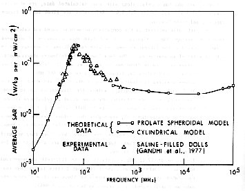
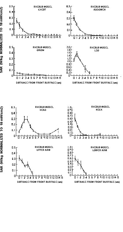
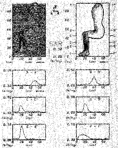
8.22. Microwave absorption profiles for rhesus monkey model

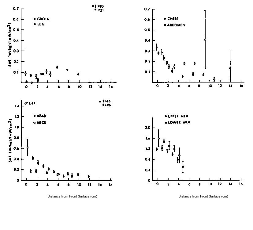
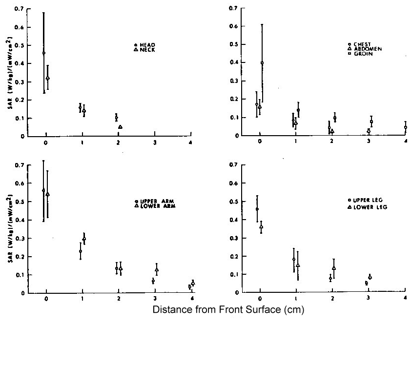
8.23. Profiles of electromagnetic absorption in the sitting rhesus model at 225 MHz

8.24. Normalized microwave absorption profiles in the man-sized model at 2.0 GHz

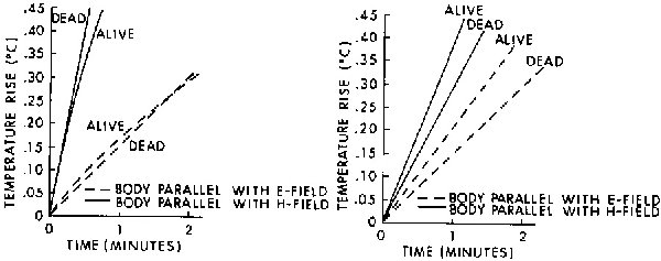
8.25. Rate of temperature rise from RFR exposure in the face of a detached M. mulatta head; 1.2 GHz, CW, 70 mW/cm², far field

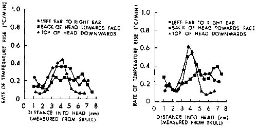
8.26. Rate of temperature rise from RFR exposure at the right side of a detached M. mulatta head; 1.2 GHz, CW, 70mW/cm², far field

8.27. Rate of temperature rise from RFR exposure at the back of a detached M. mulatta head; 1.2 GHz, CW, 70 mW/cm², far field

8.28. Rate of temperature rise from RFR exposure to the back of an M. mulatta cadaver head (with body attached); 1.2 GHz, W, 70 mW/cm ², in the far field

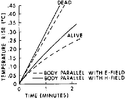
8.29. Temperature rise at 2.0 cm into the top of the head of an M. mulatta exposed to 70 mW/cm², 1.2 CHz, CW, RFR, in the far field

8.30. Temperature rise at 3.5 cm into the top of the head of an M. mulatta exposed to 70 mW/cm ², 1.2 GHz, CW, RFR, in the far field

8.31. Temperature rise at 3.5 cm into the back of the head of an M. mulatta exposed to 70 mW/cm², 1.2 GHz, CW, RFR, in the far field

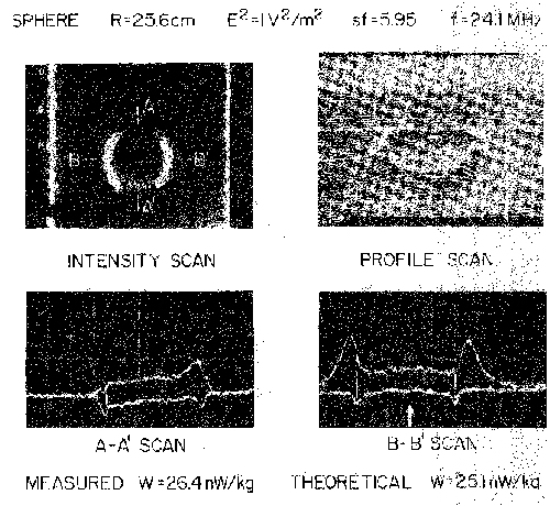
8.32. Thermographic results of exposing a 4.3-cm-radius sphere to 144-MHz TM₁₁₀ electric field in a rectangular resonant cavity simulating a 25.6-cm-radius sphere exposed to 24.1 MHz

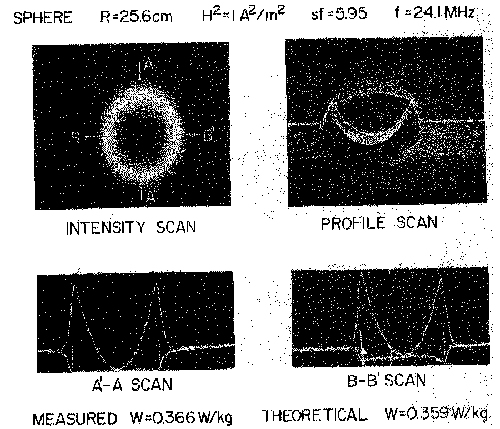
8.33. Thermographic results of exposing a 4.3-cm-radius sphere to 144-MHz TE₁₀₂ magnetic field in a rectangular resonant cavity simulating a 25.6-cm-radius sphere exposed to 24.1 MHz

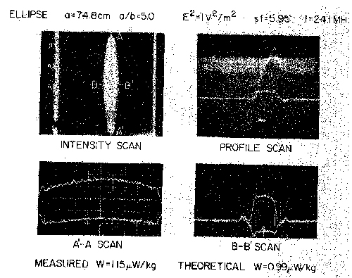
8.34. Scale-model thermograms and calculated peak SAR for 70kg, 5/1 prolate spheroid (a = 74.8 cm) exposed to 24.1-MHz electric field parallel to the major axis

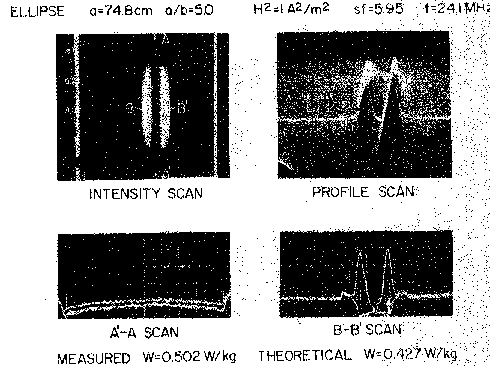
8.35. Scale-model thermograms and calculated peak SAR for 70kg, 5/1 prolate spheroid (a = 74.8 cm) exposed to 24.1- MHz magnetic field perpendicular to the major axis

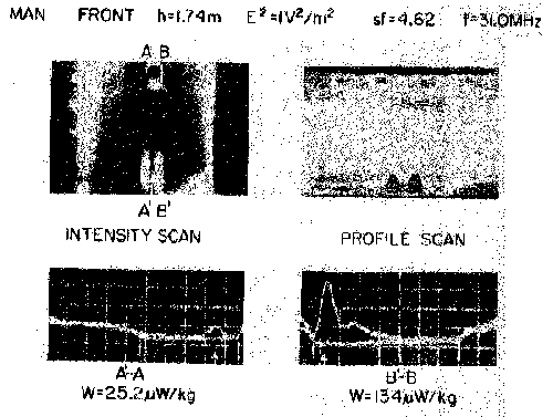
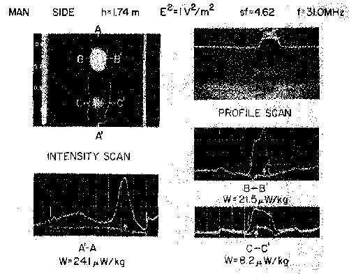
8.36. Scale-model thermograms and measured peak-SAR for 70kg, 1.74-m-height frontal-plane man model exposed to 31.0-MHz electric field parallel to the long axis

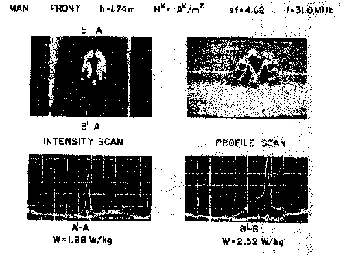
8.37. Scale-model thermograms and measured peak SAR for 70kg, 1.74-m-height frontal-plane man model exposed to 31.0-MHz magnetic field perpendicular to the major axis

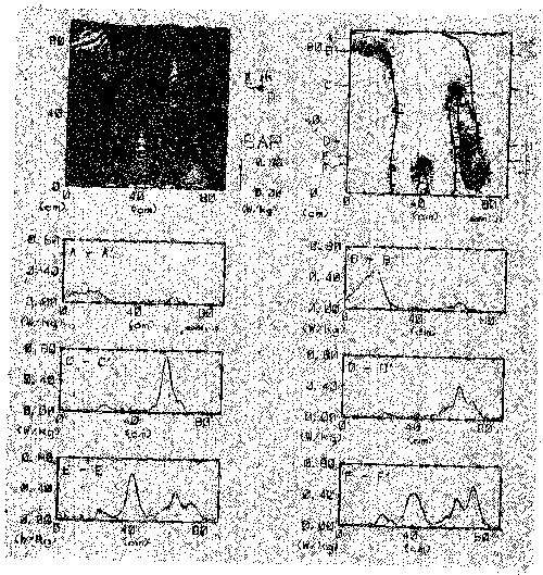
8.38. Scale-model thermograms and measured peak SAR for 70kg, 1.74-m-height medial-plane man model exposed to 31.0-MHz magnetic field perpendicular to the median plane

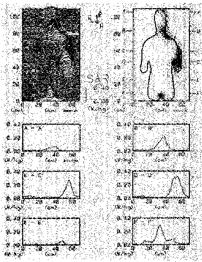
8.39. Scale-model thermograms and measured peak SAR for 70kg, 1.74-m-height medial-plane man model exposed to 31.0-MHz electric field parallel to the major axis

8.40. Computer-processed whole-body thermograms expressing 2 SAR patterns for man with arms up, exposed to 1-mW/cm² 450-MHz radiation with EHK polarization

8.41. Computer-processed whole-body thermograms expressing SAR patterns for man with one arm extended, exposed to 1-mW/cm ² 450-MHz radiation with KEH polarization

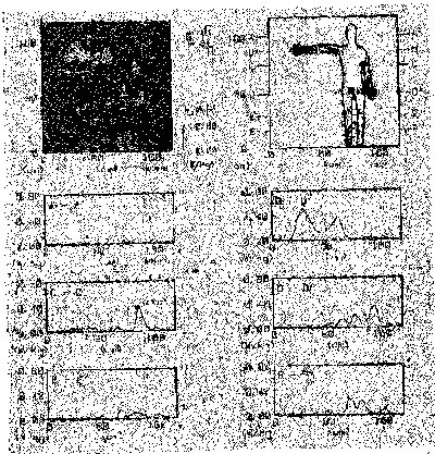
8.42. Computer-processed upper-body thermograms expressing SAR patterns for man with one arm extended, exposed to 1-mW/cm ² 450-MHz radiation with KEH polarization

8.43. Computer-processed midbody thermograms expressing SAR patterns for man with one arm extended, exposed to 1-mW/cm² 450-MHz radiation with KEH polarization

8.44. Computer-processed lower-body thermograms expressing SAR patterns for man with one arm extended, exposed 1-mW/cm² 450-MHz radiation with KEH polarization

8.45. Computer-processed whole-body thermograms expressing SAR patterns for man sitting (frontal plane), exposed to 1-mW/cm² 450-MHz radiation with EKH polarization

8.46. Computer-processed whole-body thermograms expressing SAR patterns for man sitting (sagittal plane through leg), exposed to 1-mW/cm² 450-MHz radiation with EHK polarization

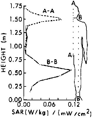
8.47. SAR distribution along an average man-model height for two cross sections; 1-mW/cm² incident-power density on the surface of the model, frequency 350 MHz E||L back to front

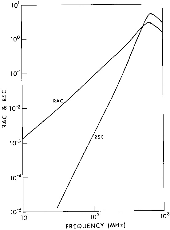
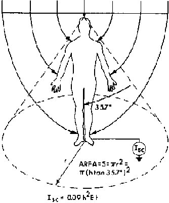
9.1. Relationship between effective area and short-circuit current for exposed human figure

9.2. Relative surface-current distribution in grounded man exposed to VLF-MF fields

9.3. Relative surface-current distribution in man exposed in free space to VLF-MF electric fields

9.4. Relative surface-current distribution in man exposed to VLF-MF electric fields with feet insulated and hand grounded

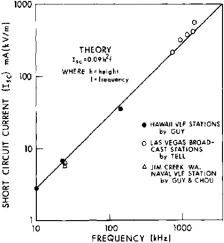
9.5. Comparison of theoretical and measured short-circuit body current of grounded man exposed to VLF-MF electric field that is parallel to body axis

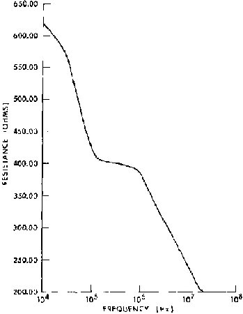
9.6. Average values of the human body resistance assumed for the calculations

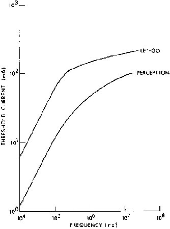
9.7. Perception and let-go currents for finger contact for a 50th percentile human as a function of frequency assumed for the calculations

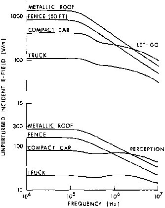
9.8. Unperturbed incident E-field required to create threshold perception and let-go currents in a human for conductive finger contact with various metallic objects,as a function of frequency

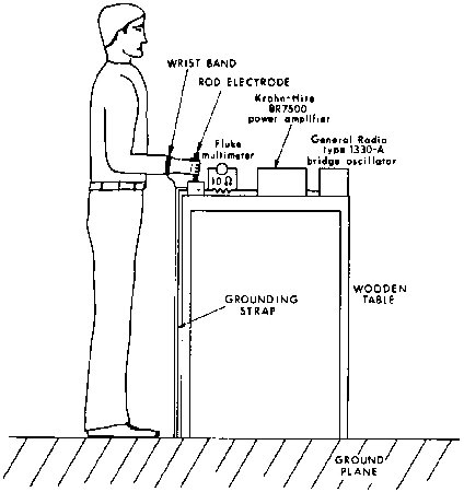
9.9. Experimental arrangement for measuring threshold currents for perception and let-go

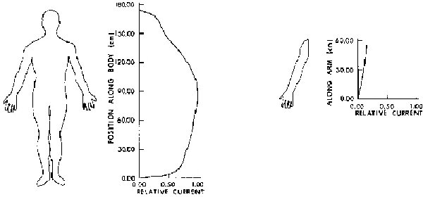
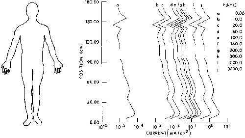
9.10. Calculated current distributions as a function of position in man exposed to 1-kV/m VLF-MF fields with feet grounded

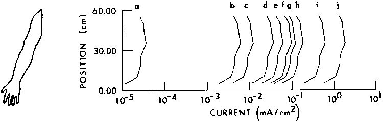
9.11. Calculated current density flowing through one arm. The exposure condition is the same as that of Figure 9.10

9.12. Calculated current distribution as a function of position in man exposed to 1-kV/m VLF-MF fields in free space

9.13. Calculated current density flowing through one arm. The exposure condition is the same as for Figure 9.12

9.14. Calculated current distributions as a function of position in man exposed to 1-kV/m VLF-MF fields with feet insulated but hands grounded

9.15. Calculated current density flowing through one arm. Exposure condition is the same as for Figure 9.14

9.16. Calculated current distribution as a function of position in man with hand contacting a large object and with feet grounded. A 1-mA current is assumed to be flowing through the arm, thorax, and legs of the subject to ground, F = 60 Hz

9.17. Calculated current density flowing through one arm. Exposure condition is same as for Figure 9.16

9.18. Real part, ', and imaginary part, ", of the dielectric constant for high-water-content tissue

9.19. Comparison of calculated average SAR (obtained from VLF analysis) with average SAR (reported in the first edition of this handbook) of average absorbed power in an ellipsoidal model of an average man

9.20. Comparison of theoretical and experimentally measured whole-body average SAR for realistic man models exposed at various frequencies

9.21. Required restrictions of VLF-MF electric field strength to prevent biological hazards related to shock, RF burns, and SAR exceeding ANSI C95.1 criteria

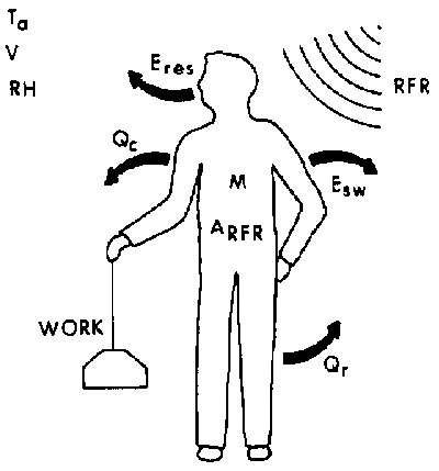
10.1. A schematic diagram of the sources of body heat (including radiofrequency radiation) and the important energy flows between man and the environment

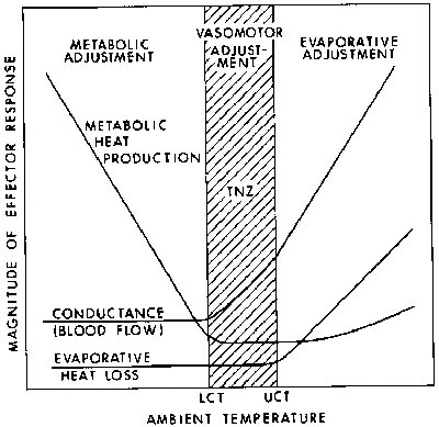
10.2. Thermoregulatory profile of a typical endothermic organism to illustrate the dependence of principal types of autonomic responses on environmental temperature

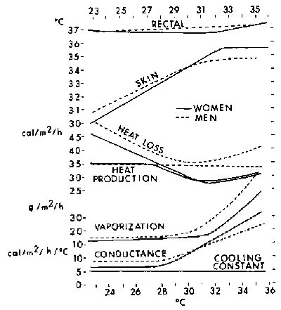
10.3. Thermoregulatory profile of nude humans equilibrated in a calorimeter to different ambient temperatures

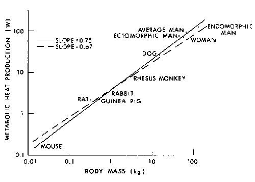
10.4. Logarithm of total metabolic heat production plotted against logarithm of body mass

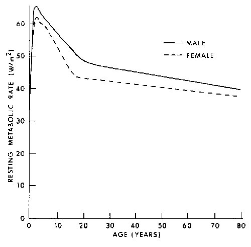
10.5. Variation of human resting metabolic rate, with age and sex, expressed as power per unit surface area

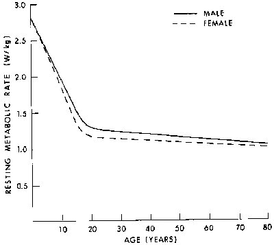
10.6. Variation of human resting metabolic rate, with age and sex, expressed as power per unit body mass

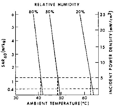
10.7. Calculated SAR₆₀ values in an average man, unclothed and quiet, irradiated by an electromagnetic planewave with E polarization at resonance (about 70 MHz)

11.1. Calculated relative RFR absorption in prolate spheroidal models of humans

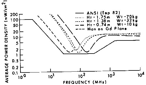
11.2. Power densities that limit human whole-body SAR to 0.4 W/kg compared to ANSI standard

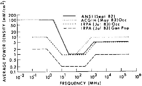
11.3. Comparison of RPR safety guidelines based on a threshold of 4 W/kg for adverse effects

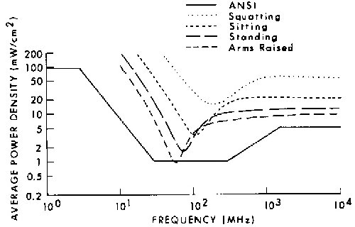
11.4. Power densities that limit human whole-body SAR to 0.4 W/kg for a 1.8-m, 70-kg person

Go to List of Tables.

Last modified: June 14, 1997
© October 1986, USAF School of Aerospace Medicine, Aerospace Medical Division (AFSC), Brooks Air Force Base, TX 78235-5301