Radiofrequency Radiation Dosimetry Handbook

6.2. CALCULATED NEAR-FIELD DOSIMETRIC DATA

FOR AVERAGE SAR

6.2.1. Short-Dipole and Small-Loop Irradiators

Figures 6.31-6.36 show the calculated average SAR in prolate spheroidal models of an average man and a medium rat irradiated by the near fields of a short electric dipole. The radiation characteristics of the dipole are shown in Figures 6.37-6.40. Figures 6.41-6.42 show the average SAR, as a function of frequency and dipole-to-body spacing, in spheroidal models of an average man exposed to the near fields of a short electric dipole and a short magnetic dipole respectively.

To emphasize the near-field absorption characteristics, the average SAR in Figures 6.31-6.36 for all frequencies is normalized to unity at a distance of one wavelength from the source. The relative SAR curves thus obtained lie close together and oscillate around the (

/d)² curve that describes the approximate variation of the far-field absorption characteristics as a function of distance from the source. Of particular interest is the possible reduction in the average SAR below the far-field value. In other words, although the reactive fields are stronger near the source, they are absorbed at a rate less than that for planewaves (far fields). This was first observed by Iskander et al., then verified experimentally and explained in terms of the variation of the incident electric and magnetic fields (Iskander et al., 1981). A detailed explanation of the relationship between the average SAR and the incident field is given in Section 3.3. These qualitative relations show that in spite of the complex characteristics of the near fields, including arbitrary angle between E and H and a wave impedance that is different from 377

, the near-field absorption characteristics can still be explained on the same basis as the far-field SARs.

Figure 6.33.
Calculated normalized average SAR as a function of the electric dipole location for E polarization in a prolate spheroidal model of an average man.

Figure 6.32.
Calculated average SAR (by long-wavelength approximation) as a function of the electric dipole location for K polarization at 27.12 MHz in a prolate spheroidal model of an average man.

Figure 6.33.
Calculated average SAR (by long-wavelength approximation) as a function of the electric dipole location for H polarization at 27.12 MHz in a prolate spheroidal model of an average man.

Figure 6.34.
Calculated average SAR (by long-wavelength approximation) as a function of the electric dipole location for E polarization at 100 MHz in a prolate spheroidal model of a medium rat.

Figure 6.35.
Calculated average SAR (by long-wavelength approximation) as a function of the electric dipole location for K polarization at 100 MHz in a prolate spheroidal model of a medium rat.

Figure 6.36.
Calculated average SAR (by long-wavelength approximation) as a function of the electric dipole location for H polarization at 100 MHz in a prolate spheroidal model of a medium rat.

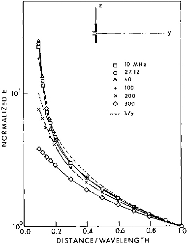
Figure 6.37. Calculated normalized E-field of a short electric dipole, as a function of y/at z = 30 cm.

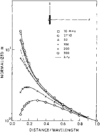
Figure 6.38. Calculated normalized H-field of a short electric dipole, as a function of y/ at z = 30 cm.

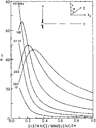
Figure 6.39. Calculated variation of as a function of y/, at z = 30 cm, for a short electric dipole.

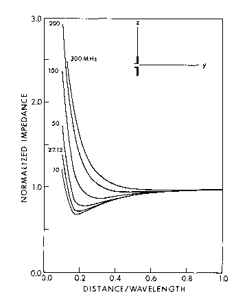
Figure 6.40. Calculated normalized field impedance of a short electric dipole, as a function of y/ at z = 30 cm.

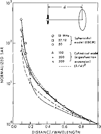
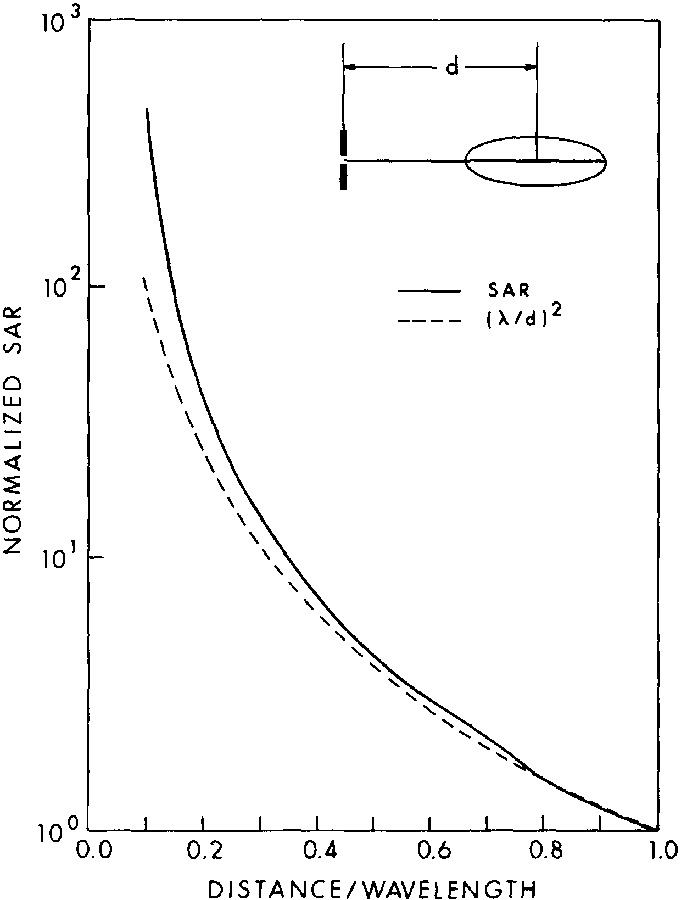
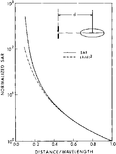
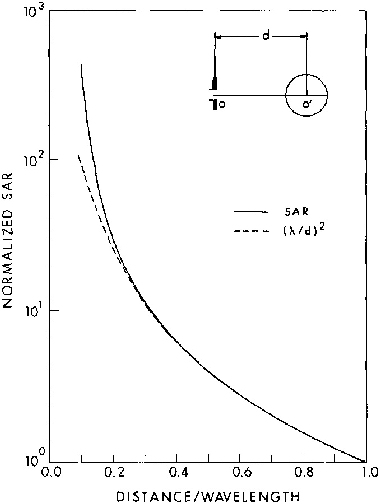
Figure 6.41. Calculated average SAR in a prolate spheroidal model of an average man irradiated by the near fields of a short electric dipole, as a function of the dipole to body spacing, d.

Figure 6.42.
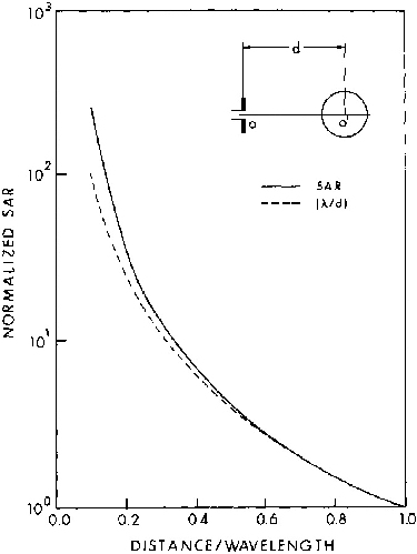
Calculated average SAR in a prolate spheroidal model of an average man irradiated by the near fields of a small magnetic dipole, as a function of the dipole-to-body spacing, d.

6.2.2. Aperture Fields

Chatterjee et al. (1980a, 1980b, 1980c) have calculated values of both local and average SARs in planar and block models of man by expressing the incident fields in terms of an angular spectrum of planewaves. Some of their data for the model of Figure 6.43 and incident E-field of Figure 6.44 are shown in Figures 6.45 and 6.46. Figure 6.44 shows the incident E_z measured near a 27.12-MHz RF sealer. They assumed no variation of the fields in the y direction, and calculated the E_xthat would satisfy Maxwell's equations for the measured E_z. Since the magnitude but not the phase of E_z was measured, they assumed that E_z had a constant phase over the measured region. Average whole-body and partial-body SAR values are shown in Figures 6.45 and 6.46 for an incident field having a half-cycle cosine variation as a function of the width of that field distribution. As the width of the aperture gets large compared to a wavelength, the SAR values approach those for an incident planewave.

To test the sensitivity of the calculations to the variation of phase of the incident field, Chatterjee et al. calculated the SARs as a function of an assumed phase variation in E_z. Figures 6.47-6.49 indicate that the SARs are not highly sensitive to the E_z phase variation. This is an important result. Measuring the phase of an incident field is difficult; if a reasonable approximation can be made on the basis of measuring only the magnitude of the incident field, near-field dosimetry will be much easier than if phase measurement is necessary. Chatterjee et al. have also compared the SARs calculated from the measured incident field and from a half-cycle cosine distribution that is a best fit to the measured field distribution. The results indicate that a reasonably approximate SAR might be obtained by using a convenient mathematical function to approximate the actual field distribution.

An important result of this work is that the calculated SARs for the incident-field distributions used in the calculations were all less than the calculated SARs for the corresponding planewave incident fields.

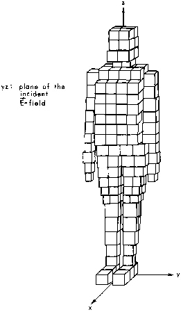
Figure 6.43.
The block model of man used by Chatterjee et al. (1980a, 1980b, 1980c) in the planewave spectrum analysis.

Figure 6.44.
Incident-field E_z from a 27.12-MHz RF sealer, used by Chatterjee et al. (1980a, 1980b, 1980c) in the planewave angular-spectrum analysis.

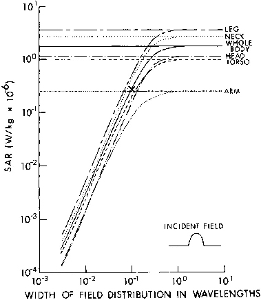
Figure 6.45.
Average whole- and part-body SAR in the block model of man placed in front of a half-cycle cosine field, E_z; frequency = 27.12 MHz, E_z|_max = 1 V/m. Calculated by Chatterjee et al. (1980a, 1980b, 1980c).

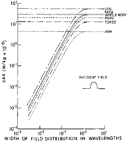
Figure 6.46.
Average whole- and part-body SAR in the block model of man placed in front of a half-cycle cosine field, E_z ; frequency = 77 MHz, E_z | _max= 1 V/m. Calculated by Chatterjee et al. (1980a, 1980b, 1980c).

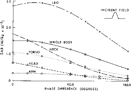
Figure 6.47.
Whole- and part-body SAR at 77 MHz in the block model of man as a function of an assumed linear antisymmetric phase variation in the incident E_z; E_z|_max = 1 V/m. Calculated by Chatterjee et al. (1980a, 1980b, 1980c).

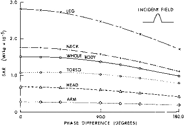
Figure 6.48.
Whole- and part-body SAR at 77 MHz in the block model of man as a function of an assumed linear symmetric phase variation in the incident E_z; E_z|_max = 1 V/m. Calculated by Chatterjee et al. (1980a, 1980b, 1980c).

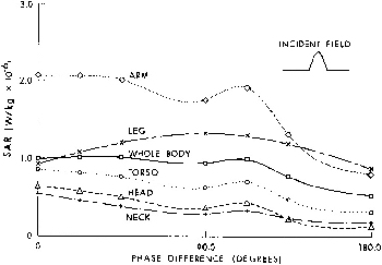
Figure 6.49. Whole- and part-body SAR at 350 MHz in the block model of man as a function of an assumed linear antisymmetric phase variation in the incident E_z; E_z |_max = 1 V/m. Calculated by Chatterjee et al. (1980a, 1980 b , 1980c).

Go to Chapter 7.1

Return to Table of Contents.

Last modified: June 14, 1997
© October 1986, USAF School of Aerospace Medicine, Aerospace Medical Division (AFSC), Brooks Air Force Base, TX 78235-5301

6.2. CALCULATED NEAR-FIELD DOSIMETRIC DATA FOR AVERAGE SAR

6.2.1. Short-Dipole and Small-Loop Irradiators

Figure 6.33. Calculated normalized average SAR as a function of the electric dipole location for E polarization in a prolate spheroidal model of an average man.

Figure 6.32. Calculated average SAR (by long-wavelength approximation) as a function of the electric dipole location for K polarization at 27.12 MHz in a prolate spheroidal model of an average man.

Figure 6.33. Calculated average SAR (by long-wavelength approximation) as a function of the electric dipole location for H polarization at 27.12 MHz in a prolate spheroidal model of an average man.

Figure 6.34. Calculated average SAR (by long-wavelength approximation) as a function of the electric dipole location for E polarization at 100 MHz in a prolate spheroidal model of a medium rat.

Figure 6.35. Calculated average SAR (by long-wavelength approximation) as a function of the electric dipole location for K polarization at 100 MHz in a prolate spheroidal model of a medium rat.

Figure 6.36. Calculated average SAR (by long-wavelength approximation) as a function of the electric dipole location for H polarization at 100 MHz in a prolate spheroidal model of a medium rat.