4.2.2. Low-Frequency Techniques
Figure 4.6.
Bridge circuit for measuring dielectric properties of materials at frequencies below 100 MHz.
The bridge is like a Wheatstone bridge, but impedances are measured instead of resistance. Balancing the bridge requires adjusting one or more of the impedances (Z1, Z2, and Z3). If the complex permittivity of the material under test is given by
![]() * =
* = ![]() o (
o (![]() ' - j
' - j![]() ") (Equation 4.6)
") (Equation 4.6)
where ![]() o is the permittivity of free space, the admittance Y of the capacitor is given by Y = j
o is the permittivity of free space, the admittance Y of the capacitor is given by Y = j![]() C. For a
lossy capacitor filled with the dielectric material under test,
C. For a
lossy capacitor filled with the dielectric material under test,
Y = j![]() K
K![]() o (
o (![]() ' - j
' - j ![]() ") (Equation 4.7)
") (Equation 4.7)
where K is a constant dependent on the geometry of the sample holder. For example, K = A/d for an ideal parallel-plate capacitor, where A is the area of the plates and d is the separation between the plates. The imaginary and real parts of the admittance are hence given by
B = ![]() K
K![]() o
o![]() ' (Equation 4.8)
' (Equation 4.8)
G = ![]() K
K![]() o
o![]() " (Equation 4.9)
" (Equation 4.9)
4.2.3. High-Frequency Techniques
Figure 4.7.
Experimental setup for measuring S-parameters, using an automatic network analyzer.
With the reflection (S11) and transmission (S12) parameters measured, the real and imaginary parts of the complex permittivity
![]() (Equation 4.10)
(Equation 4.10)
![]() (Equation 4.11)
(Equation 4.11)
where Im means imaginary part; Re, real part; ![]() , the complex reflection coefficient assuming the sample to be of infinite length; and P, the propagation factor.
, the complex reflection coefficient assuming the sample to be of infinite length; and P, the propagation factor. ![]() and P are given in terms of the S-parameters by
and P are given in terms of the S-parameters by
![]() (Equation 4.12)
(Equation 4.12)
where
 (Equation 4.13)
and
![]() (Equation 4.14)
(Equation 4.14)
where ![]() is the propagation constant and L is the length of the sample under test . This measurement procedure
provides enough information to obtain the complex permeability of the sample as well as the complex permittivity. To avoid resonance effects in these measurements, the sample length should be limited to less than a quarter of a wavelength at the highest frequency of operation. Typical sample holders suitable for these measurements at microwave frequencies are shown in Figure 4.8. For the lumped-capacitor holder in Figure 4.8b, only measurement of the reflection coefficient is required; and the calculations are made as described in the following section.
is the propagation constant and L is the length of the sample under test . This measurement procedure
provides enough information to obtain the complex permeability of the sample as well as the complex permittivity. To avoid resonance effects in these measurements, the sample length should be limited to less than a quarter of a wavelength at the highest frequency of operation. Typical sample holders suitable for these measurements at microwave frequencies are shown in Figure 4.8. For the lumped-capacitor holder in Figure 4.8b, only measurement of the reflection coefficient is required; and the calculations are made as described in the following section.
Figure 4.8.
Typical sample holders for measuring the dielectric properties of biological substances at microwave
frequencies.
(a) Coaxial sample holder.
(b) Lumped capacitor terminating a section of a coaxial transmission line.
4.2.4. Time-Domain Measurements
Figure 4.9.
Typical experimental setup for time-domain measurement of complex permittivities.
 (Equation 4.15)
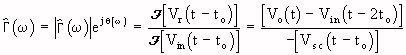
where  represents the Fourier transform; Vin and Vr, the incident and reflected voltages respectively; Vsc, the
reflected voltage when the sample holder is replaced by a short circuit; Vo, the total voltage signal recorded on the TDR screen; and to, the propagation time between the sampling probe and the sample holder. The real and imaginary parts of the relative permittivity are calculated from the complex reflection coefficient in Equation 4.15 using the following relations:
represents the Fourier transform; Vin and Vr, the incident and reflected voltages respectively; Vsc, the
reflected voltage when the sample holder is replaced by a short circuit; Vo, the total voltage signal recorded on the TDR screen; and to, the propagation time between the sampling probe and the sample holder. The real and imaginary parts of the relative permittivity are calculated from the complex reflection coefficient in Equation 4.15 using the following relations:
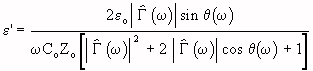 (Equation 4.16)
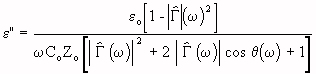 (Equation 4.17)
where ![]() and
and ![]() are, respectively, the magnitude and phase of the frequency-domain reflection coefficient, and Co is the capacitance of the airfilled capacitor terminating the transmission line of characteristic impedance Zo.
are, respectively, the magnitude and phase of the frequency-domain reflection coefficient, and Co is the capacitance of the airfilled capacitor terminating the transmission line of characteristic impedance Zo.
4.2.5. Measurement of in Vivo Dielectric Properties
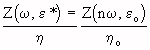 (Equation 4.18)
where
Z = antenna impedance
![]() * = complex permittivity of the material being measured
* = complex permittivity of the material being measured
 = intrinsic impedance of the material being measured
![]() = intrinsic impedance of free space
= intrinsic impedance of free space
![]() = index of refraction of the material being measured relative to free space
= index of refraction of the material being measured relative to free space
Figure 4.10.
In vivo dielectric probes for measuring dielectric properties of biological substances.
(a) Open-ended section of coaxial transmission line.
(b) A short electric monopole immersed in the material under test.
(c) The low-frequency (neglecting radiation resistance) equivalent circuits.
When a short monopole antenna is used as the probe, the probe impedance is given by
 (Equation 4.19)
where A and C are constants determined by the probe's dimensions. This expression is valid when the probe
length is less than 10% of the wavelength in the material being measured. Combining this expression with Equation 4.18 gives the following expressions for the resistance and reactance of the complex impedance Z(![]() ,
, ![]() *) = R + jX:
*) = R + jX:
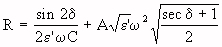 (Equation 4.20)
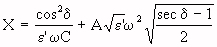
where tan ![]() is the loss tangent. In the above pair of equations all parameters except
is the loss tangent. In the above pair of equations all parameters except  ' and
' and ![]() are known or
can be determined from experimental measurements. Because simultaneous solution of these equations is difficult, an iterative method of solution is usually used. The second terms in Equations 4.20 and 4.21 are small at low
frequencies. When these terms are neglected, the following equations result:
are known or
can be determined from experimental measurements. Because simultaneous solution of these equations is difficult, an iterative method of solution is usually used. The second terms in Equations 4.20 and 4.21 are small at low
frequencies. When these terms are neglected, the following equations result:
 (Equation 4.22)
 (Equation 4.23)
Solutions to these equations are obtained by dividing Equation 4.22 by 4.23 to get tan  = R/X; therefore,
by measuring the input impedance of a short monopole antenna inserted into a material, we can calculate both the relative dielectric constant,
= R/X; therefore,
by measuring the input impedance of a short monopole antenna inserted into a material, we can calculate both the relative dielectric constant, ![]() ', and the conductivity,
', and the conductivity, ![]() .
.
C (
- A rigorous expression developed by Wu (1963) is used for the input impedance of the in vivo probe immersed in the material under test. The method of analysis, therefore, accounts for the radiation resistance of the probe for larger values of h/
 , where h is the length of the center-conductor extension, and is the wavelength.
- Because the mathematical expressions for this case are very complex, the dielectric parameters of the sample under test are determined by comparing the measured and calculated values of the input impedance, using an iterative two-dimensional (error surface) complex zerofinding routine. This procedure is illustrated graphically in Figure 4.11 (Olson and Iskander, 1986).
Figure 4.11.
Graphical illustration of the iterative procedure for calculating complex permittivity parameters by
minimizing the difference between measured and calculated values of the input impedance of the in vivo dielectric
probe. The minimum on the error surface | Z measured - Z calculated | indicates the most appropriate values ' and " that satisfy the measured value of the input impedance.
4.2.6. Summary
![]()
Go to Chapter 4.3
Return to Table of Contents.
Last modified: June 24, 1997
© October 1986, USAF School of Aerospace Medicine, Aerospace Medical Division (AFSC), Brooks Air Force Base, TX 78235-5301